Data cleaning and feature processing

Data often has missing values and some abnormal points, which need to be processed to continue the subsequent analysis or modeling. Therefore, the first step to get the data is to clean the data. In this task, we will learn the operations such as missing values, duplicate values, string and data conversion to clean the data into a form that can be analyzed or modeled.

2.1 observation data and processing

2.1.1 missing value observation

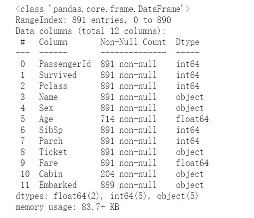
#FA Yi
df.info()

#Method 2
df.isnull().sum()

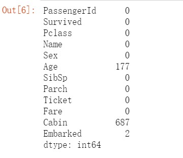
You can see that Age, cabin and embanked all have missing values

2.1.2 task 2: deal with missing values

#Three ways to set NAN to 0
df[df['Age']==None]=0
df[df['Age'].isnull()] = 0 
df[df['Age'] == np.nan] = 0

None is a NoneType

np.nan is not an "empty" object. To judge whether a value is empty, you can only use NP IsNaN (I) function.
np.nan is a non empty object whose type is the basic data type float.
np.nan() can perform null value detection on either DataFrame, Python list or just a value. But generally in practical application, NP Nan () is mostly used to check a single value.

pd.isnull() can perform null value detection on either DataFrame, Python list or just a value. But generally in practical application, PD Isnull() is used to verify a DataFrame or Series.

Note: in this data, after reading the data in the numerical column, the data type of the vacant value is float64, so it is generally impossible to use None for indexing, and NP is best used for comparison nan

df.dropna().head(3)
df.fillna(0).head(3)

Function name	describe
dropna	The axis labels are filtered according to whether the value of each label is missing data, and the threshold is determined according to the allowable missing data
fillna	Fill in missing data with some values or use interpolation ('fill ',' bfill ')

2.2 repeated observation and treatment

2.2.1 viewing duplicate values in data

df[df.duplicated()]

2.2.2 processing of duplicate values

#Examples of methods for cleaning up the entire row with duplicate values:
df=df.drop_duplicates()

2.2.3 save the previously cleaned data in csv format

df.to_csv('test_clear.csv')

2.3 feature observation and treatment

The above data are mainly divided into
Numerical features: Survived, Pclass, Age, SibSp, Parch, Fare. Among them, Survived and Pclass are discrete numerical features, and Age, SibSp, Parch, Fare are continuous numerical features
Text type features: Name, Sex, Cabin, embossed, Ticket, among which Sex, Cabin, embossed, Ticket are category type text features

Numerical features can generally be directly used for model training, but sometimes continuous variables are discretized for the sake of model stability and robustness. Text features often need to be converted into numerical features before they can be used for modeling and analysis.

2.3.1 box (discretization) processing of age ¶

(1) What is the sub box operation?

(2) The continuous variable Age was divided into five Age groups and represented by category variable 12345

(3) The continuous variable Age is divided into five Age groups [0,5) [5,15] [15,30) [30,50) [50,80], which are represented by category variable 12345 respectively

(4) The continuous variable Age was divided into five Age groups: 10%, 30%, 50%, 70%, 90%, and expressed by the categorical variable 12345

(5) Save the data obtained above in csv format

#The continuous variable Age was divided into five Age groups and represented by category variable 12345
df['AgeBand']=pd.cut(df['Age'],5,labels=[1,2,3,4,5])

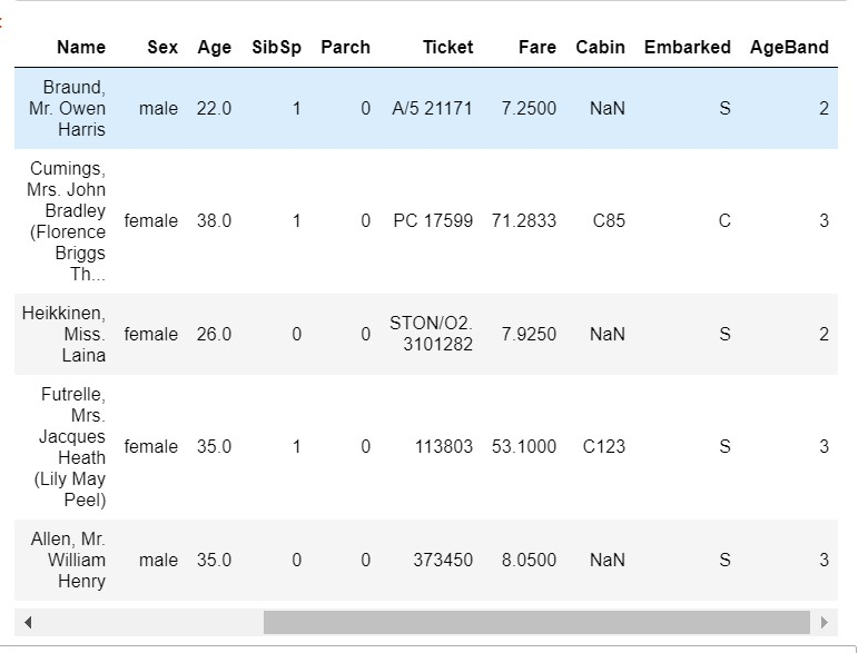
#The continuous variable Age is divided into five Age groups [0,5) [5,15] [15,30) [30,50) [50,80], which are represented by category variable 12345 respectively
df['AgeBand'] = pd.cut(df['Age'],[0,5,15,30,50,80],labels = [1,2,3,4,5])
df.head(3)
#The continuous variable Age was divided into five Age groups of 10% 30% 50 70% 90% and expressed by the categorical variable 12345
df['AgeBand'] = pd.qcut(df['Age'],[0,0.1,0.3,0.5,0.7,0.9],labels = [1,2,3,4,5])
df.head()

2.3.2 converting text variables

(1) View text variable name and type
(2) Text variables Sex, Cabin and embanked are represented by numerical variables 12345
(3) The text variables Sex, Cabin and embanked are represented by one hot coding

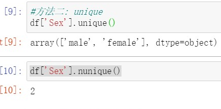
#View category text variable name and category

#Method 1: value_counts
df['Sex'].value_counts()
df['Cabin'].value_counts()
#Method 2: unique
df['Sex'].unique()
df['Sex'].nunique()

unique() returns all unique values of a column (all unique values of a feature) in the form of an array (numpy.ndarray)
nunique() is the number of unique values returned

#Convert category text to 12345

#Method 1: replace
df['Sex_num'] = df['Sex'].replace(['male','female'],[1,2])
df.head()
#Method 2: map
df['Sex_num'] = df['Sex'].map({'male': 1, 'female': 2})
df.head()
#Method 3: use sklearn LabelEncoder for preprocessing
from sklearn.preprocessing import LabelEncoder
for feat in ['Cabin', 'Ticket']:
    lbl = LabelEncoder()  
    label_dict = dict(zip(df[feat].unique(), range(df[feat].nunique())))
    df[feat + "_labelEncode"] = df[feat].map(label_dict)
    df[feat + "_labelEncode"] = lbl.fit_transform(df[feat].astype(str))

#Convert category text to one hot encoding

#Method 1: OneHotEncoder
for feat in ["Age", "Embarked"]:
#     x = pd.get_dummies(df["Age"] // 6)
#     x = pd.get_dummies(pd.cut(df['Age'],5))
    x = pd.get_dummies(df[feat], prefix=feat)
    df = pd.concat([df, x], axis=1)
    #df[feat] = pd.get_dummies(df[feat], prefix=feat)

2.3.3 extract the features of Titles from the Name features of plain text (the so-called Titles are Mr,Miss,Mrs, etc.)

df['Title'] = df.Name.str.extract('([A-Za-z]+)\.', expand=False)
df.head()