In my last article article In this paper, I introduce the concept of graph neural network (GNN) and some of its latest developments. As this topic becomes more and more exaggerated, I decided to make this tutorial to introduce how to easily implement your graph neural network in the project. You will learn how to use pytorch geometry to build your own GNN and how to use GNN to solve a real-world problem (Recsys Challenge 2015).
In this blog post, we will use PyTorch and PyTorch geometry (pyg), a very fast graph neural network framework based on PyTorch. It is several times faster than the most famous GNN framework DGL.
In addition to the amazing speed, PyG also comes with a series of well implemented GNN models, which are described in various papers. Therefore, it will be very convenient to reproduce these experiments with PyG.
Given its advantages in speed and convenience, PyG is undoubtedly one of the most popular and widely used GNN libraries. Let's discuss this topic in depth and practice it for ourselves
Requirements
- PyTorch — 1.1.0
- PyTorch Geometric — 1.2.0
PyTorch Geometric Basics
This section will take you through the basics of PyG. Basically, it will override torch_geometric.data and torch_geometric.nn. You will learn how to transfer geometric data to your GNN and how to design a custom MessagePassing layer, the core of GNN.
Data
torch_ The geometric. Data module contains a data class that allows you to easily create graphs from data. You only need to specify:
- Attributes / properties associated with each node
- Connectivity / adjacency of each node (edge index)
Connectivity / adjacency of each node (edge index)
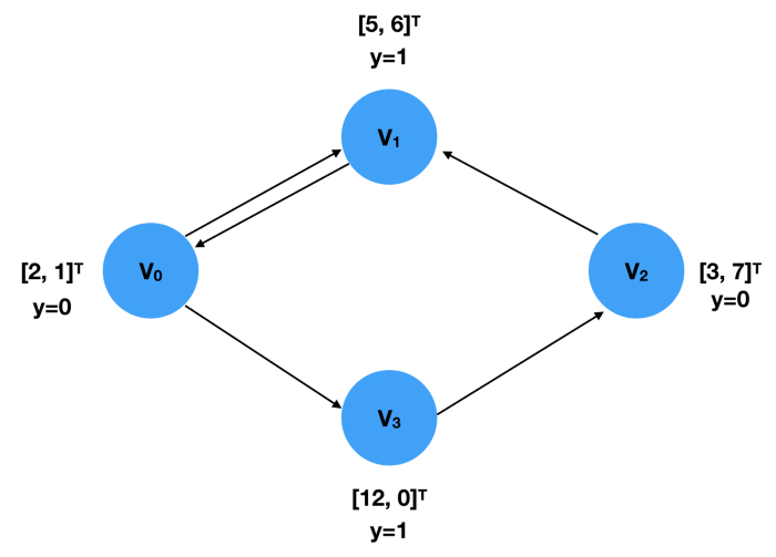
In the figure, there are four nodes, V1 and V4. Each node is associated with a two-dimensional eigenvector, and the label y represents its category. These two can be expressed as FloatTensors:
x = torch.tensor([[2,1], [5,6], [3,7], [12,0]], dtype=torch.float)
y = torch.tensor([0, 1, 0, 1], dtype=torch.float)
The connectivity (edge index) of the graph should be limited to COO format, that is, the first list contains the index of the source node, and the second list specifies the index of the target node.
edge_index = torch.tensor([[0, 1, 2, 0, 3],
                           [1, 0, 1, 3, 2]], dtype=torch.long)
Note that the order of the edge indexes is independent of the Data object created, because this information is only used to calculate the adjacency matrix. Therefore, the edge above_ The information represented by index is the same as below.
edge_index = torch.tensor([[0, 2, 1, 0, 3],
                           [3, 1, 0, 1, 2]], dtype=torch.long)
Put them together, we can create Data objects as follows:
import torch
from torch_geometric.data import Data


x = torch.tensor([[2,1], [5,6], [3,7], [12,0]], dtype=torch.float)
y = torch.tensor([0, 1, 0, 1], dtype=torch.float)

edge_index = torch.tensor([[0, 2, 1, 0, 3],
                           [3, 1, 0, 1, 2]], dtype=torch.long)


data = Data(x=x, y=y, edge_index=edge_index)
>>> Data(edge_index=[2, 5], x=[4, 2], y=[4])
Dataset
The data set creation process is not very simple, but for those who have used torch vision, it may look familiar because PyG follows its convention. PyG provides two different types of dataset classes, InMemoryDataset and dataset. As you can literally see, the former is used for data suitable for RAM, while the latter is used for larger data. Because their implementations are very similar, I will only discuss InMemoryDataset.
To create an InMemoryDataset object, you need to implement four functions
- raw_file_names()
It returns a list showing an original, unprocessed list of file names. If you have only one file, the returned list should contain only one element. In fact, you can simply return an empty list and specify your file in process().
- processed_file_names()
Similar to the previous function, it also returns a list of file names containing all processed data. After calling process(), usually, the returned list should have only one element, storing the unique processed data file name.
- download()
This function should download the data you are processing to self. Raw_ Directory specified in dir. If you don't need to download data, just visit
pass
In a function.
- process()
This is the most important method of data set. You need to collect data into the data object list. Then, self.collate() is called to calculate the slice that the DataLoader object will use. Here is an example from PyG official website An example of a custom dataset for.
import torch
from torch_geometric.data import InMemoryDataset


class MyOwnDataset(InMemoryDataset):
    def __init__(self, root, transform=None, pre_transform=None):
        super(MyOwnDataset, self).__init__(root, transform, pre_transform)
        self.data, self.slices = torch.load(self.processed_paths[0])

    @property
    def raw_file_names(self):
        return ['some_file_1', 'some_file_2', ...]

    @property
    def processed_file_names(self):
        return ['data.pt']

    def download(self):
        # Download to `self.raw_dir`.

    def process(self):
        # Read data into huge `Data` list.
        data_list = [...]

        if self.pre_filter is not None:
            data_list [data for data in data_list if self.pre_filter(data)]

        if self.pre_transform is not None:
            data_list = [self.pre_transform(data) for data in data_list]

        data, slices = self.collate(data_list)
        torch.save((data, slices), self.processed_paths[0])
Later in this article, I will show how to create a custom dataset from the data provided in RecSys Challenge 2015.
DataLoader
The DataLoader class allows you to easily batch feed data into your model. To create a DataLoader object, simply specify the Dataset and the required batch size.
loader = DataLoader(dataset, batch_size=512, shuffle=True)
Each iteration of the DataLoader object produces a batch object, which is very similar to the Data object, but has a batch attribute. It indicates which graph each node is associated with. Because the DataLoader will be x, y, and edge from different samples / graphs_ The index is aggregated into a batch, so the GNN model needs this batch information to know which nodes belong to the same graph in a batch, so as to perform calculations.
for batch in loader:
    batch
    >>> Batch(x=[1024, 21], edge_index=[2, 1568], y=[512], batch=[1024])
MessagePassing
Message passing is the essence of GNN. It describes how to learn node embedding. I discussed it in the last article, so I'll briefly introduce the terms that conform to PyG documents.
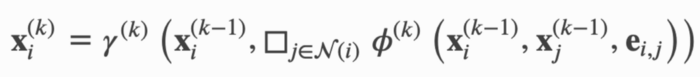
x represents node embedding, e represents edge characteristics, 휙 represents message function, aggregation function, and 훾 represents update function. If the edges in a graph have no other characteristics except connectivity, e is essentially the edge index of the graph. Superscript indicates the index of the layer. When k=1, x represents the input characteristics of each node. Next, I'll explain how each function works
- propagate(edge_index, size=None, **kwargs):
It accepts edge indexes and other optional information, such as node characteristics (embedding). Calling this function will therefore call messages and updates.
- message(**kwargs):
You can specify how messages are constructed for each node pair (x_i, x_j). Since it follows the call of propagate, it can accept any parameter passed to propagate. One thing to note is that you can use_ I and_ J defines the mapping from parameters to specific nodes. Therefore, you must be very careful when naming the parameters of this function.
- update(aggr_out, **kwargs)
It accepts the aggregate message and other parameters passed to the propagate and assigns a new embedded value to each node.
Example
Let's see how to implement the SageConv layer from the paper Inductive representation learning map . The message passing formula of SageConv is defined as:
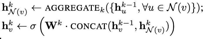
Here, we use the maximum pool as the aggregation method. Therefore, the right side of the first line can be written as

It illustrates how messages are constructed. The embedding of each adjacent node is multiplied by a weight matrix, plus an offset, and through an activation function. This can be easily done with torch.nn.Linear.
class SAGEConv(MessagePassing):
    def __init__(self, in_channels, out_channels):
        super(SAGEConv, self).__init__(aggr='max')
        self.lin = torch.nn.Linear(in_channels, out_channels)
        self.act = torch.nn.ReLU()

    def message(self, x_j):
        # x_j has shape [E, in_channels]

        x_j = self.lin(x_j)
        x_j = self.act(x_j)

        return x_j
The update section aggregates the aggregated message and the current node embedding. Then multiply by another weight matrix and apply another activation function.
class SAGEConv(MessagePassing):
    def __init__(self, in_channels, out_channels):
        super(SAGEConv, self).__init__(aggr='max')
        self.update_lin = torch.nn.Linear(in_channels + out_channels, in_channels, bias=False)
        self.update_act = torch.nn.ReLU()

    def update(self, aggr_out, x):
        # aggr_out has shape [N, out_channels]

        new_embedding = torch.cat([aggr_out, x], dim=1)
        new_embedding = self.update_lin(new_embedding)
        new_embedding = torch.update_act(new_embedding)

        return new_embedding
Put it together, we have the SageConv layer below.
import torch
from torch.nn import Sequential as Seq, Linear, ReLU
from torch_geometric.nn import MessagePassing
from torch_geometric.utils import remove_self_loops, add_self_loops
class SAGEConv(MessagePassing):
    def __init__(self, in_channels, out_channels):
        super(SAGEConv, self).__init__(aggr='max') #  "Max" aggregation.
        self.lin = torch.nn.Linear(in_channels, out_channels)
        self.act = torch.nn.ReLU()
        self.update_lin = torch.nn.Linear(in_channels + out_channels, in_channels, bias=False)
        self.update_act = torch.nn.ReLU()

    def forward(self, x, edge_index):
        # x has shape [N, in_channels]
        # edge_index has shape [2, E]


        edge_index, _ = remove_self_loops(edge_index)
        edge_index, _ = add_self_loops(edge_index, num_nodes=x.size(0))


        return self.propagate(edge_index, size=(x.size(0), x.size(0)), x=x)

    def message(self, x_j):
        # x_j has shape [E, in_channels]

        x_j = self.lin(x_j)
        x_j = self.act(x_j)

        return x_j

    def update(self, aggr_out, x):
        # aggr_out has shape [N, out_channels]


        new_embedding = torch.cat([aggr_out, x], dim=1)

        new_embedding = self.update_lin(new_embedding)
        new_embedding = self.update_act(new_embedding)

        return new_embedding
A Real-World Example — RecSys Challenge 2015
The 2015 RecSys challenge challenged data scientists to establish a conference based recommendation system. This challenge requires participants to complete two tasks:
- Predict whether there will be a purchase event, followed by a series of clicks
- Predict what to buy
First, we start with RecSys Challenge 2015 official website Download the data and build the Dataset. We'll start with the first task because it's easier.
The above official website was hung up (November 28, 2021), but it can be downloaded from Kaggle Download from.
The challenge provides two main sets of data, including click events and purchase events, namely yoochoose click. DAT and yoochoose buy. Dat. Let's take a quick look at the data:
Preprocessing
After downloading the data, we preprocess it to provide it to our model. item_ The ID is classified and encoded to ensure the encoded item_ The ID (which will be mapped to the embedding matrix later) starts at 0.
from sklearn.preprocessing import LabelEncoder
import pandas as pd
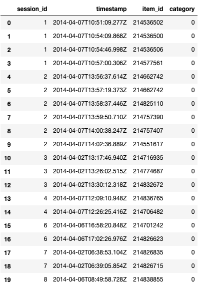
df = pd.read_csv('../input/yoochoose-clicks.dat', header=None)
df.columns=['session_id','timestamp','item_id','category']
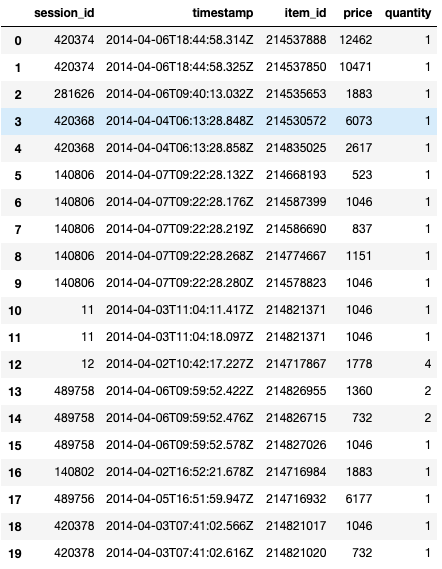
buy_df = pd.read_csv('../input/yoochoose-buys.dat', header=None)
buy_df.columns=['session_id','timestamp','item_id','price','quantity']
item_encoder = LabelEncoder()
df['item_id'] = item_encoder.fit_transform(df.item_id)
df.head()
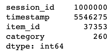
Because the data is quite large, we sub sampled it for easier demonstration.
#randomly sample a couple of them
sampled_session_id = np.random.choice(df.session_id.unique(), 1000000, replace=False)
df = df.loc[df.session_id.isin(sampled_session_id)]
df.nunique()
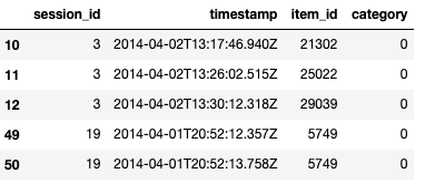
To determine the basic fact, that is, whether there is a given session for any purchase event, we just need to check whether the session is in yoochoose click. Dat_ Id also appears in yoochoose buy. Dat.
df['label'] = df.session_id.isin(buy_df.session_id)
df.head()
[external chain picture transfer failed. The source station may have anti-theft chain mechanism. It is recommended to save the picture and upload it directly (img-njci56pz-1638088147507)( https://miro.medium.com/max/422/1 *A5jaCXd41plzf8Fvva3_tA.png#pic_center)]
Dataset Construction
After the preprocessing step is completed, the data can be converted into a Dataset object. Here, we treat each item in the session as a node, so all items in the same session form a graph. To build the Dataset, we use session_id groups the preprocessed data and traverses the groups. In each iteration, the items in each group_ ID is classified and encoded again, because for each graph, the node index should be counted from 0. Therefore, we have the following contents:
import torch
from torch_geometric.data import InMemoryDataset
from tqdm import tqdm

class YooChooseBinaryDataset(InMemoryDataset):
    def __init__(self, root, transform=None, pre_transform=None):
        super(YooChooseBinaryDataset, self).__init__(root, transform, pre_transform)
        self.data, self.slices = torch.load(self.processed_paths[0])

    @property
    def raw_file_names(self):
        return []
    @property
    def processed_file_names(self):
        return ['../input/yoochoose_click_binary_1M_sess.dataset']

    def download(self):
        pass

    def process(self):

        data_list = []

        # process by session_id
        grouped = df.groupby('session_id')
        for session_id, group in tqdm(grouped):
            sess_item_id = LabelEncoder().fit_transform(group.item_id)
            group = group.reset_index(drop=True)
            group['sess_item_id'] = sess_item_id
            node_features = group.loc[group.session_id==session_id,['sess_item_id','item_id']].sort_values('sess_item_id').item_id.drop_duplicates().values

            node_features = torch.LongTensor(node_features).unsqueeze(1)
            target_nodes = group.sess_item_id.values[1:]
            source_nodes = group.sess_item_id.values[:-1]

            edge_index = torch.tensor([source_nodes, target_nodes], dtype=torch.long)
            x = node_features

            y = torch.FloatTensor([group.label.values[0]])

            data = Data(x=x, edge_index=edge_index, y=y)
            data_list.append(data)

        data, slices = self.collate(data_list)
        torch.save((data, slices), self.processed_paths[0])
After building the data set, we call shuffle() to ensure that it has been shuffled randomly, and then divide it into three sets for training, verification and testing.
dataset = dataset.shuffle()
train_dataset = dataset[:800000]
val_dataset = dataset[800000:900000]
test_dataset = dataset[900000:]
len(train_dataset), len(val_dataset), len(test_dataset)
Build a Graph Neural Network
The following custom GNN references An example from PyG's official Github repository . I changed the GraphConv layer to the self implementing SAGEConv layer shown above. In addition, the output layer is also modified to match the binary classification settings.
embed_dim = 128
from torch_geometric.nn import TopKPooling
from torch_geometric.nn import global_mean_pool as gap, global_max_pool as gmp
import torch.nn.functional as F
class Net(torch.nn.Module):
    def __init__(self):
        super(Net, self).__init__()

        self.conv1 = SAGEConv(embed_dim, 128)
        self.pool1 = TopKPooling(128, ratio=0.8)
        self.conv2 = SAGEConv(128, 128)
        self.pool2 = TopKPooling(128, ratio=0.8)
        self.conv3 = SAGEConv(128, 128)
        self.pool3 = TopKPooling(128, ratio=0.8)
        self.item_embedding = torch.nn.Embedding(num_embeddings=df.item_id.max() +1, embedding_dim=embed_dim)
        self.lin1 = torch.nn.Linear(256, 128)
        self.lin2 = torch.nn.Linear(128, 64)
        self.lin3 = torch.nn.Linear(64, 1)
        self.bn1 = torch.nn.BatchNorm1d(128)
        self.bn2 = torch.nn.BatchNorm1d(64)
        self.act1 = torch.nn.ReLU()
        self.act2 = torch.nn.ReLU()

    def forward(self, data):
        x, edge_index, batch = data.x, data.edge_index, data.batch
        x = self.item_embedding(x)
        x = x.squeeze(1)

        x = F.relu(self.conv1(x, edge_index))

        x, edge_index, _, batch, _ = self.pool1(x, edge_index, None, batch)
        x1 = torch.cat([gmp(x, batch), gap(x, batch)], dim=1)

        x = F.relu(self.conv2(x, edge_index))

        x, edge_index, _, batch, _ = self.pool2(x, edge_index, None, batch)
        x2 = torch.cat([gmp(x, batch), gap(x, batch)], dim=1)

        x = F.relu(self.conv3(x, edge_index))

        x, edge_index, _, batch, _ = self.pool3(x, edge_index, None, batch)
        x3 = torch.cat([gmp(x, batch), gap(x, batch)], dim=1)

        x = x1 + x2 + x3

        x = self.lin1(x)
        x = self.act1(x)
        x = self.lin2(x)
        x = self.act2(x)
        x = F.dropout(x, p=0.5, training=self.training)

        x = torch.sigmoid(self.lin3(x)).squeeze(1)

        return x
Training
Training our custom GNN is very simple. We simply iterate the DataLoader constructed from the training set and back propagate the loss function. Here, we use Adam as the optimizer, the learning rate is set to 0.005, and the binary cross entropy is used as the loss function.
def train():
    model.train()

    loss_all = 0
    for data in train_loader:
        data = data.to(device)
        optimizer.zero_grad()
        output = model(data)
        label = data.y.to(device)
        loss = crit(output, label)
        loss.backward()
        loss_all += data.num_graphs * loss.item()
        optimizer.step()
    return loss_all / len(train_dataset)

device = torch.device('cuda')
model = Net().to(device)
optimizer = torch.optim.Adam(model.parameters(), lr=0.005)
crit = torch.nn.BCELoss()
train_loader = DataLoader(train_dataset, batch_size=batch_size)
for epoch in range(num_epochs):
    train()
Validation
This tag is highly unbalanced with a large number of negative tags, because there are no purchase events after most sessions. In other words, a stupid model that guesses all the negatives will give you more than 90% accuracy. Therefore, area under curve (AUC) is a better measure for this task, because it only cares whether the score of positive examples is higher than that of negative examples. We use Sklearn's ready-made AUC calculation function.
def evaluate(loader):
    model.eval()

    predictions = []
    labels = []

    with torch.no_grad():
        for data in loader:

            data = data.to(device)
            pred = model(data).detach().cpu().numpy()

            label = data.y.detach().cpu().numpy()
            predictions.append(pred)
            labels.append(label)
Result
I trained the model for one stage and measured the AUC scores of training, verification and test
for epoch in range(1):
    loss = train()
    train_acc = evaluate(train_loader)
    val_acc = evaluate(val_loader)
    test_acc = evaluate(test_loader)
    print('Epoch: {:03d}, Loss: {:.5f}, Train Auc: {:.5f}, Val Auc: {:.5f}, Test Auc: {:.5f}'.
          format(epoch, loss, train_acc, val_acc, test_acc))

With only 1 million lines of training data (about 10% of all data) and 1 training epoch, we can obtain the AUC score of the verification and test set of about 0.73. If more data and larger training steps are used to train the model, the score is likely to improve.
Conclusion
You have learned the basic usage of PyTorch geometry, including dataset construction, custom layers, and training gnn with real data. All the code in this article can also be found in My Github repo You can find another Jupyter notebook file where I solved the second task of the 2015 RecSys challenge. I hope you like this article. If you have any questions or comments, please leave a message below! Be sure to twitter Follow me on, where I share my blog posts or interesting machine learning / in-depth learning news! Did GNN and PyG have fun