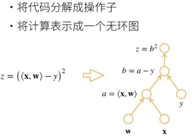
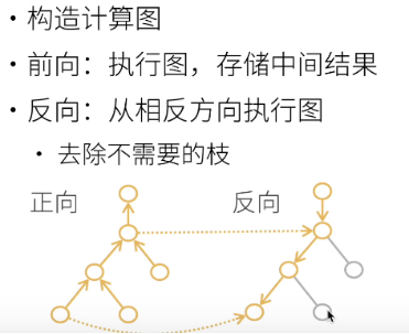
1, Calculation diagram

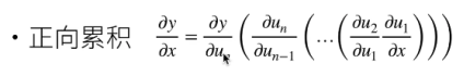
1. Forward

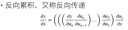
2. Reverse


3. Complexity
The computational complexity of both forward and reverse is O (n). Because you need to traverse the graph to calculate the gradient.
The memory complexity in the forward direction is O (1), while that in the reverse direction is O (n), because the reverse direction requires one pass in the forward direction to save the intermediate value, which takes up space.

2, Structure

1. Display structure (Tensorflow/theano/MXNet)
First construct the formula (calculation diagram), and then bring it into numerical calculation. Generally, it belongs to display structure mathematically.
2. Implicit construction (pytorch/MXNet)
Write the program flow chart directly, and then the framework constructs the calculation chart in the background

It is not difficult to find from the above that pytorch is implicitly constructed, which means that gradient calculation can only call reverse derivation, and the previous composition is calculated in reverse

3, Automatic derivation code usage

1. Assuming y=2xTx, take the derivative with respect to the column vector X
(1) Sir, form a vector

import torch

x = torch.arange(4.)

(2) Storage gradient
Before calculating the gradient of y with respect to x, you need a place to store the gradient. Use requirements first_ grad_ (true) indicates that the gradient needs to be saved and then stored in grad.

x.requires_grad_(True) # Intermediate results need to be stored
x.grad # View the gradient of x, which defaults to None

(3) Calculate y

y = 2*torch.dot(x,x) # Dot product
y # tensor(28., grad_fn=<MulBackward0>)

dot for inner product. 11+22+33+44=28.
Y is an implicitly constructed computational graph, so y has a gradient function with grad_fn inside.

(4) Call back propagation function

y.backward() # Back propagation of y
x.grad # View the gradient obtained by BP


(backpropagation: Back propagation)

x.grad==4*x #Tensor ([true, true, true]) indicates that the derivative of y is 4*x

2. Calculate the next function related to x
Clean up x.grad and re-enter the accumulation of function y equal to X.
x.grad_ zero_ () # the gradient of pytoch will accumulate. Here, write 0 to the gradient

y = x.sum() 
y.backward() # Back propagation of y
x.grad #tensor([1.,1.,1.,1.])

Why should y assume the transpose of x times x instead of x times x?
Because for vector x, xTx is equivalent to twice the dot product, which is a scalar, and x*x is a matrix. Deep learning is generally to find the reciprocal of scalar.
For non scalar calls to "backward", you need to pass in a "gradient" parameter. Generally, non scalars are summed and backward is called.

Why sum and call the backward function?
Because sum is the sum of this function, using the chain rule, first the derivative becomes 2x, and then the derivative of sum (x). X is a vector. After taking the derivative of X, it is a vector with all 1, multiplied by 2x. The final result is a vector that is all 2x.

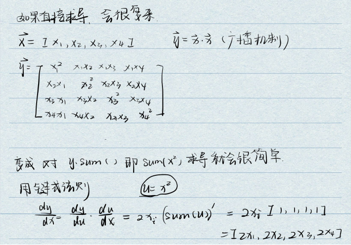
x.grad_zero_()
y = x*x
y.sum().backward()# Equivalent to x*x == sum(y · y)
x.grad #tensor([0.,2.,4.,6.])

3. Move the calculation out of the calculation diagram

# Move the calculation out of the calculation diagram
x.grad_zero_()
y = x*x  
u = y.detach() #If you drop ydetach, then u is a constant, and the value is x*x
z = u*x  #The constant times the vector, and the last z is still a vector
z.sum().backward()  #To derive a vector, you need to call sum to become a scalar first
x.gard==u #tensor([True,True,True,True])
detach It is useful in some places where network parameters need to be fixed, such as loss Derivative of.

4. To build the calculation diagram of the function in time, we need to control the flow through Python, and we can still calculate the gradient of the variable

def f(a):
    b = a * 2
    while b.norm() < 1000:
        b = b * 2
    if b.sum() > 0:
        c = b
    else:
        c = 100 * b
    return c

# Mr. Torch generates a calculation diagram and saves the intermediate value to facilitate back propagation.
# A generates a random number randn. size = () indicates that a is a scalar and the gradient requires needs to be recorded_ grad=True. 
a = torch.randn(size=(), requires_grad=True)
d = f(a)
d.backward()

# f() can be understood as a flow of calculation diagram, and finally get d
# From the above function, we can see that it is a linear function, and its gradient is the slope d/a
a.grad == d / a

5. Test code

import torch

x = torch.arange(4.)
x.requires_grad_(True) # Intermediate results need to be stored
# The above two formulas are equivalent to x = torch arange(4.,requires_grad=True)
x.grad # View the gradient of x, which defaults to None

y = 2*torch.dot(x,x) # Point scale
y # tensor(28., grad_fn=<MulBackward0>)

y.backward() # Back propagation of y
x.grad # View the gradient obtained by BP

# y=2x^2 y'=2x, you can judge whether the gradient obtained by BP is correct
4*x == x.grad

x.grad_zero_() # The gradient of Pytorch will accumulate. Here is the vector that rewrites x as all zeros, the last one_ It means re
y = x.sum() # sum() after derivation is equivalent to dot multiplying a vector with all 1 
y.backward()
x.grad

x.grad_zero_()
y = x*x
# x*x == sum(y·y)
y.sum().backward()
x.grad


# Move the calculation out of the calculation diagram
x.grad_zero_()
y = x*x
u = y.detach()
z = u*x

z.sum().backward()
x.gard==u

# To build the calculation diagram of the function in time, we need to control the flow through Python, and we can still calculate the gradient of the variable
def f(a):
    b = a * 2
    while b.norm() < 1000:
        b = b * 2
    if b.sum() > 0:
        c = b
    else:
        c = 100 * b
    return c
# size = () scalar
a = torch.randn(size=(), requires_grad=True)
d = f(a)
d.backward()
a.grad == d / a