catalogue
1. Basic concept of Hassi Watch
2.2 division and remainder method
2.3 several less commonly used methods
1. Basic concept of Hassi Watch
Hash table (Hash table, also known as Hash table) is accessed directly according to the key value data structure . That is, it accesses records by mapping key values to a location in the table to speed up the search. This mapping function is called Hash function , storage of records array be called Hash table.
Given table M, there is a function f(key). For any given keyword value key, after substituting into the function, if the address recorded in the table containing the keyword can be obtained, table M is called Hash table, and function f(key) is Hash function------ From Baidu.
There are many places in life where Hassi watches are used, such as:
1. Learning English when we encounter a word we don't know when learning English, we always check the word online:
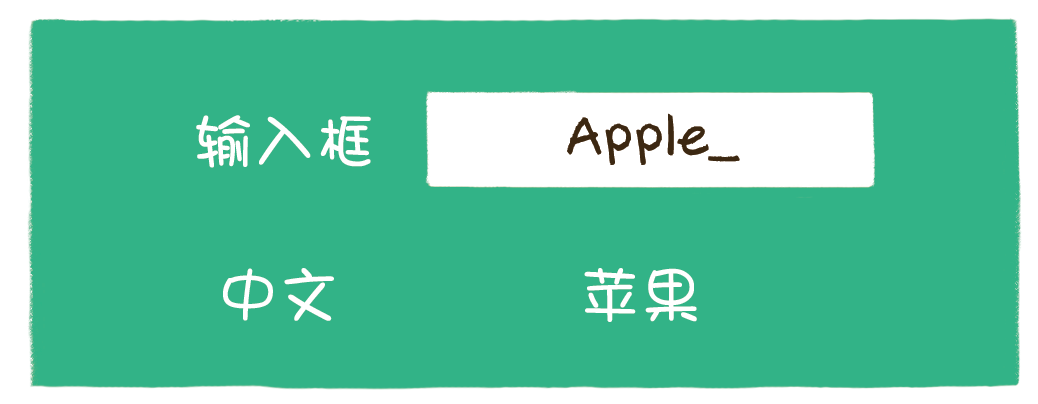
Although English teachers do not recommend this, because the Chinese data found in the electronic dictionary is too limited, while the traditional paper dictionary can find a variety of meanings, parts of speech, example sentences and so on. But personally, I prefer this way
In our program world, we often need to store such a "dictionary" in memory to facilitate our efficient query and statistics.
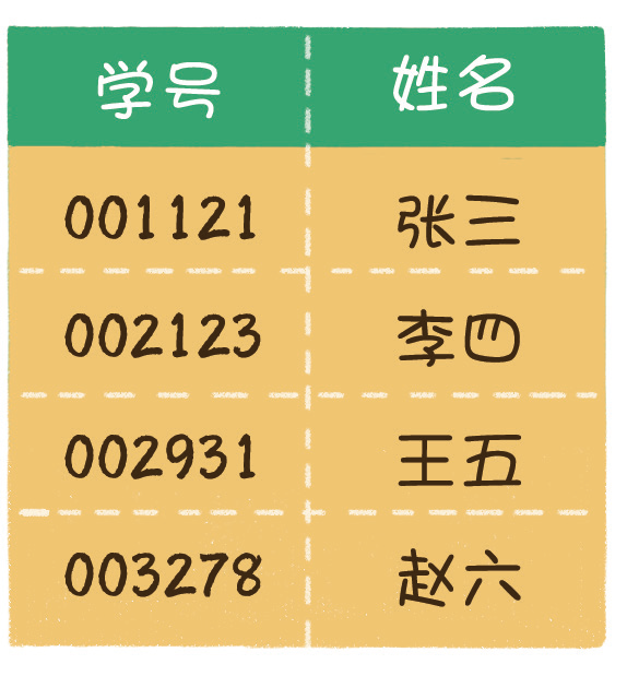
For example, developing a student management system requires the function of quickly finding out the name of the corresponding student by entering the student number. There is no need to query the database every time, but a cache table can be established in memory, which can improve the query efficiency.
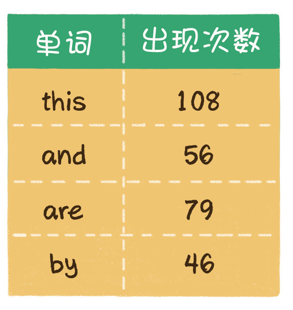
For another example, if we need to count the frequency of some words in an English book, we need to traverse the contents of the whole book and record the times of these words in memory.
Because of these requirements, an important data structure was born. This data structure is called hash table, also known as hashtable.
The process of inserting and searching elements into Hassy table is as follows:
1. Insert element
According to the key of the element to be inserted, this function calculates the storage location of the element and stores it according to this location
2. Search elements
Carry out the same calculation for the key code of the element, take the obtained function value as the storage location of the element, and take the element ratio according to this location in the structure
If the keys are equal, the search is successful.
Bihasi function
2.1 direct setting method
Direct customization method: take a linear function of the keyword as the Hash address: Hash (Key) = A*Key + B
1. Advantages: simple and uniform
2. Disadvantages: you need to know the distribution of keywords in advance and only use those with a relatively small range
3. Usage scenario: suitable for finding small and continuous situations
4. Not applicable scenario: when the data distribution is relatively scattered, such as 1199847348, 90 and 5, this method is not suitable
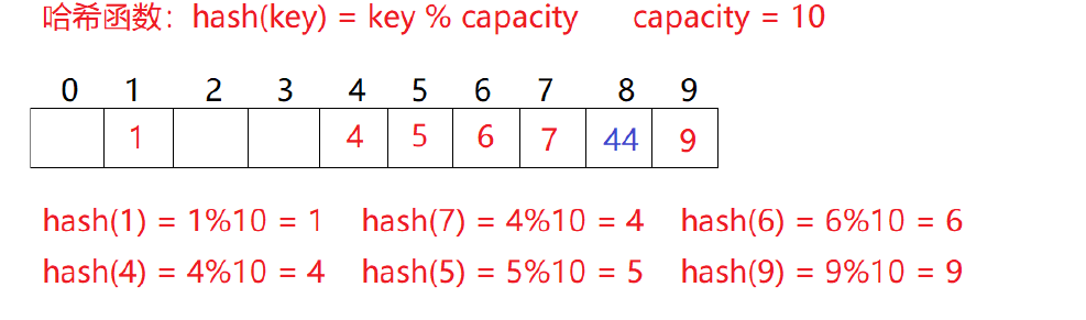
2.2 division and remainder method
Divide and leave remainder method: set the number of addresses allowed in the hash table as m, take a prime number p not greater than m but closest to or equal to m as the divisor, and convert the key code into hash address according to the hash function: hash (key) = key% p (p < = m)
Advantages: wide range of use, basically unlimited.
Disadvantages: there is Hassi conflict, which needs to be solved. When there are many Hassi conflicts, the efficiency decreases very severely.
2.3 several less commonly used methods
1. Square middle method
hash(key)=key*key, and then take the middle digits of the function return value as the Hassy address
Assuming that the keyword is 1234, its square is 1522756, and the middle three bits 227 are extracted as the hash address; For another example, if the keyword is 4321, its square is 18671041, and the middle three bits 671 (or 710) are extracted as the hash address.
The square median method is more suitable: do not know the distribution of keywords, and the number of digits is not very large
2. Folding method
The folding method is to divide the keyword from left to right into several parts with equal digits (the digits of the last part can be shorter), then overlay and sum these parts, and take the last few digits as the hash address according to the length of the hash table. The folding method is suitable for the situation that there is no need to know the distribution of keywords in advance and there are many keywords
3. Random number method
Select a random function and take the random function value of the keyword as its hash address, that is, H(key) = random(key), where random is a random number function.
4. Mathematical analysis
There are n d digits, and each bit may have r different symbols. The frequency of these r different symbols may not be the same in each bit. They may be evenly distributed in some bits, and the opportunities of each symbol are equal. They are unevenly distributed in some bits, and only some symbols often appear. According to the size of the hash table, we can select several bits in which various symbols are evenly distributed as the hash address. Assuming that the employee registration form of a company is to be stored, if the mobile phone number is used as the keyword, it is very likely that the first seven bits are the same, then we can select the last four bits as the hash address. If such extraction is still prone to conflict, The extracted numbers can also be reversed (for example, 1234 is changed to 4321), the right ring displacement (for example, 1234 is changed to 4123), the left ring displacement, and the superposition of the first two numbers and the last two numbers (for example, 1234 is changed to 12 + 34 = 46).
Digital analysis method is usually suitable for dealing with the situation of large number of keywords, if the distribution of keywords is known in advance and several bits of keywords are evenly distributed
III. Hassi conflict
Hassi conflict means that different key s calculate the same Hassi mapping address through the same Hassi function. This phenomenon is called Hassi conflict. Here is an example:
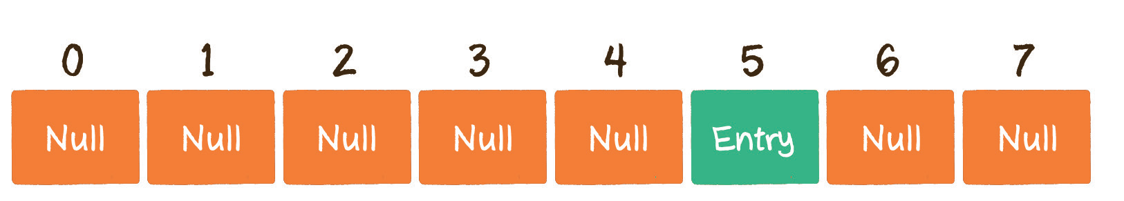
First, we insert a set of Key Value pairs with # Key # 002931 and # Value # Wang Wu. What exactly should I do?
Step 1: convert # Key # into array subscript # 5 through hash function.
Step 2: if there is no element in the position corresponding to the array subscript 5, fill the # Entry # into the position of the array subscript 5 #.
However, due to the limited length of the array, when more and more entries are inserted, the subscripts obtained by different keys through the hash function may be the same. For example, the index of the array corresponding to the Key 002936 is 2; 002947 the index of the array corresponding to this Key is also 2.
This situation is called hash conflict. Alas, the hash function "hits the shirt". What should I do?
Hash conflicts cannot be avoided. Since they cannot be avoided, we must find a way to solve them. There are two main methods to solve hash conflict, one is open addressing method, the other is linked list method.
Four open address method
4.1 linear detection
Open addressing is also called closed hashing.
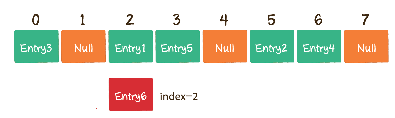
The principle of the open addressing method is very simple. When a Key obtains the corresponding array index through the hash function and has been occupied, we can "find another job" to find the next neutral position.
Taking the above situation as an example, Entry6 obtains the subscript 2 through the hash function. If the subscript already has other elements in the array, move it back by 1 bit to see if the position of the array subscript 3 is empty.
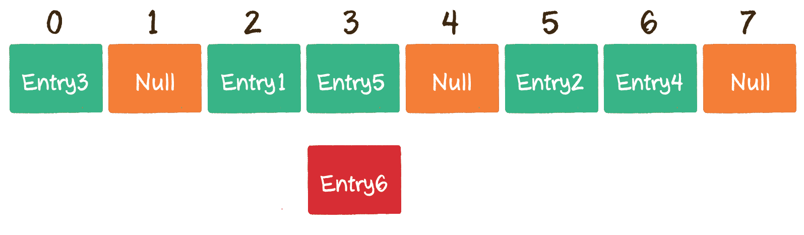
Unfortunately, the subscript , 3 , has also been occupied. Then move the , 1 , bit backward to see if the position of the subscript , 4 , of the array is empty.
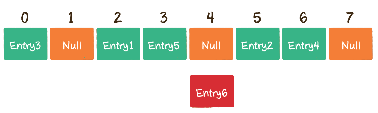
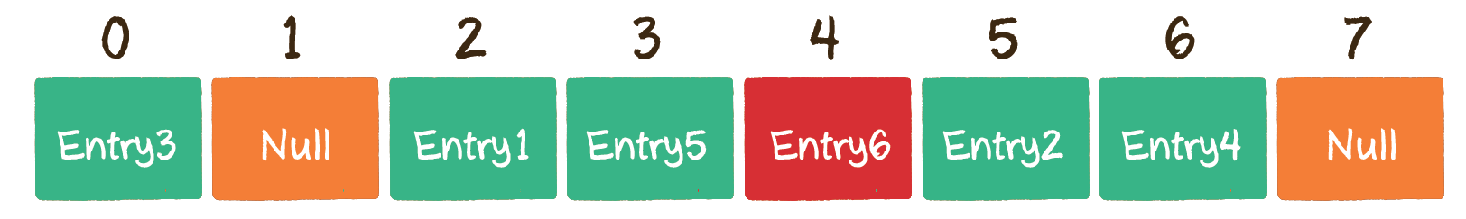
Fortunately, the position of the array subscript , 4 , has not been occupied, so , Entry6 , is stored in the position of the array subscript , 4 ,.
We can find that the more data in Hassi table, the more serious Hassi conflict. In addition, the hash table is implemented based on array, so the hash table also involves the problem of capacity expansion
When the hash is expressed to a certain saturation after multiple element insertion, the probability of Key mapping position conflict will gradually increase. In this way, a large number of elements are crowded in the same array subscript position to form a long linked list, which has a great impact on the performance of subsequent insertion and query operations. At this time, the hash table needs to expand its length, that is, expand its capacity.
Under what circumstances can the hash table be expanded? How to expand capacity? Here, the load factor of hash table is defined as: α = Fill in the number of elements in the table / the length of the hash table α It is a marker factor of hash table fullness. Since the meter length is a fixed value, α It is directly proportional to the "number of elements filled in the table", so, α The larger the, the more elements filled in the table, the greater the possibility of conflict; conversely, α The smaller the, the fewer elements marked in the table, and the less likely there is to be a conflict. In fact, the average lookup length of hash table is a function of load factor o, but different conflict handling methods have different functions.
For the open addressing method, the load factor is a particularly important factor and should be strictly limited to less than 0.7-0.8. If it exceeds 0.8, the CPU cache miss during table lookup increases according to the exponential curve. Therefore, some hash libraries using open addressing method, such as Java system libraries, limit the load factor to 0.75. If it exceeds this value, it will resize the hash table.
4.2 secondary detection
The defect of linear detection is that conflicting data are stacked together, which has something to do with finding the next empty position, because the way to find the empty position is to find it one by one next to each other. Therefore, in order to avoid this problem, the method of finding the next empty position for secondary detection is: H, = (Ho + I2)% m, or h, = (Ho - I2)% M. Where: i=1,2,3, H is the position obtained by calculating the key of the element through the hash function Hash(x), and M is the size of the table. If 44 is to be inserted in 2.1, there is a conflict. The situation after use is solved as follows:
The research shows that when the length of the table is a prime number and the table loading factor A does not exceed 0.5, the new table entry can be inserted, and any position will not be explored twice. Therefore, as long as there are half empty positions in the table, there will be no problem of full table. When searching, you can not consider the situation that the table is full, but when inserting, you must ensure that the loading factor a of the table does not exceed 0.5. If it exceeds, you must consider increasing the capacity.
Corresponding code:
Here we explain how to find the hash table:
Find the corresponding value of # Entry # with # Key # 002936 # in the hash table. What exactly should I do? Let's take the linked list method as an example.
Step 1: convert Key into array subscript 2 through hash function.

Step 2: find the element corresponding to array subscript 2. If the Key of this element is 002936, it will be found; If the Key is not 002936, it doesn't matter. Continue to look back from the next position. If the next position is empty, it means there is no number. If the last position of the array is found, continue to look back from the beginning.
#pragma once
#include <vector>
#include <iostream>
using namespace std;

namespace CloseHash
{
	enum State
	{
		EMPTY,
		EXITS,
		DELETE,
	};

	template<class K, class V>
	struct HashData
	{
		pair<K, V> _kv;
		State _state = EMPTY;  // state
	};

	template<class K>
	struct Hash
	{
		size_t operator()(const K& key)
		{
			return key;
		}
	};

	// Specialization
	template<>
	struct Hash<string>
	{
		// "int"  "insert"
		// The string is converted to a corresponding integer value, because the mapping position can be obtained only by integer
		// The expected - > string is different, and the transferred out integer value should be different as far as possible
		// "abcd" "bcad"
		// "abbb" "abca"
		size_t operator()(const string& s)
		{
			// BKDR Hash
			size_t value = 0;
			for (auto ch : s)
			{
				value += ch;
				value *= 131;
			}

			return value;
		}
	};

	template<class K, class V, class HashFunc = Hash<K>>
	class HashTable
	{
	public:
		bool Insert(const pair<K, V>& kv)
		{
			HashData<K, V>* ret = Find(kv.first);
			if (ret)
			{
				return false;
			}

			// If the load factor is greater than 0.7, the capacity will be increased
			//if (_n*10 / _table.size() > 7)
			if (_table.size() == 0)
			{
				_table.resize(10);
			}
			else if ((double)_n / (double)_table.size() > 0.7)
			{
				//vector<HashData> newtable;
				// newtable.resize(_table.size*2);
				//for (auto& e : _table)
				//{
				//	if (e._state == EXITS)
				//	{
				//		//Recalculate and put into newtable
				//		// ... Similar to the insertion logic below
				//	}
				//}

				//_table.swap(newtable);

				HashTable<K, V, HashFunc> newHT;
				newHT._table.resize(_table.size() * 2);
				for (auto& e : _table)
				{
					if (e._state == EXITS)
					{
						newHT.Insert(e._kv);
					}
				}

				_table.swap(newHT._table);
			}

			HashFunc hf;
			size_t start = hf(kv.first) % _table.size();
			size_t index = start;

			// Position behind detection -- linear detection or secondary detection
			size_t i = 1;
			while (_table[index]._state == EXITS)
			{
				index = start + i;
				index %= _table.size();
				++i;
			}

			_table[index]._kv = kv;
			_table[index]._state = EXITS;
			++_n;

			return true;
		}

		HashData<K, V>* Find(const K& key)
		{
			if (_table.size() == 0)
			{
				return nullptr;
			}

			HashFunc hf;
			size_t start = hf(key) % _table.size();//Take out the key value by using the imitation function. It is possible that the key does not support modulo
			size_t index = start;
			size_t i = 1;
			while (_table[index]._state != EMPTY)//Not empty, continue to find
			{
				if (_table[index]._state == EXITS
					&& _table[index]._kv.first == key)//eureka
				{
					return &_table[index];
				}

				index = start + i;
				index %= _table.size();
				++i;
			}

			return nullptr;
		}

		bool Erase(const K& key)
		{
			HashData<K, V>* ret = Find(key);
			if (ret == nullptr)
			{
				return false;
			}
			else
			{
				ret->_state = DELETE;
				return true;
			}
		}

	private:
		/*	HashData* _table;
			size_t _size;
			size_t _capacity;*/
		vector<HashData<K, V>> _table;
		size_t _n = 0;  // Number of valid data stored
	};
Five zipper method
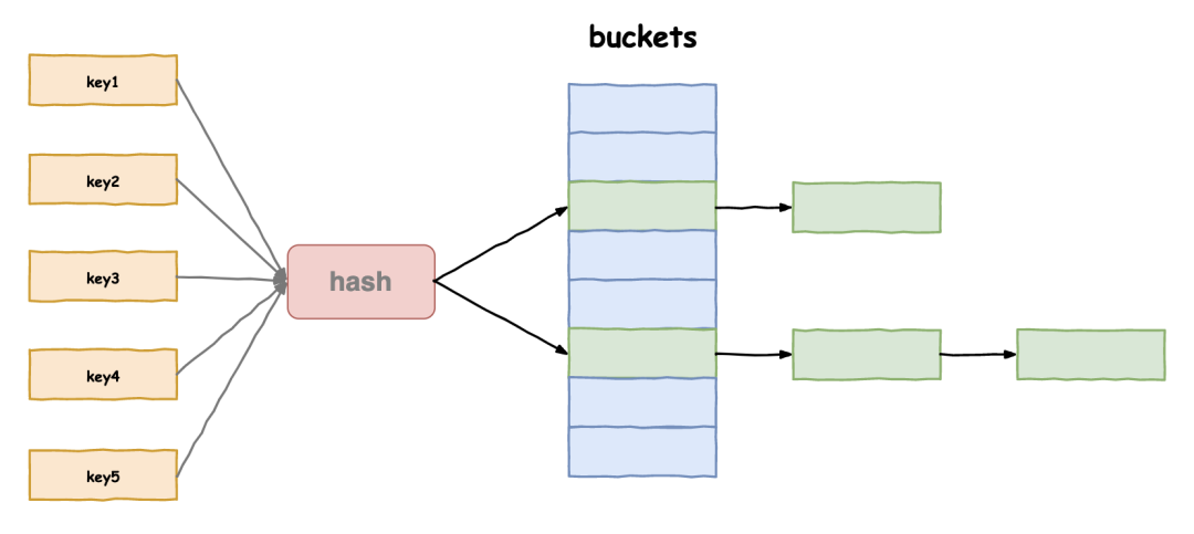
1. Open hash concept
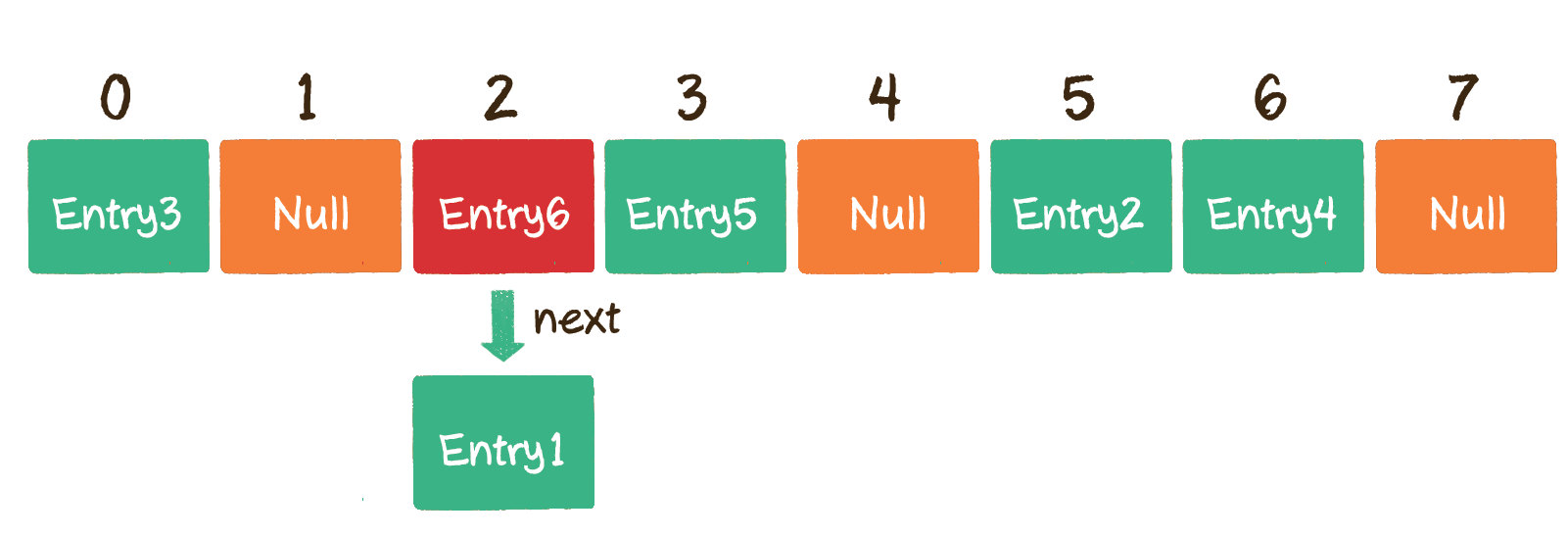
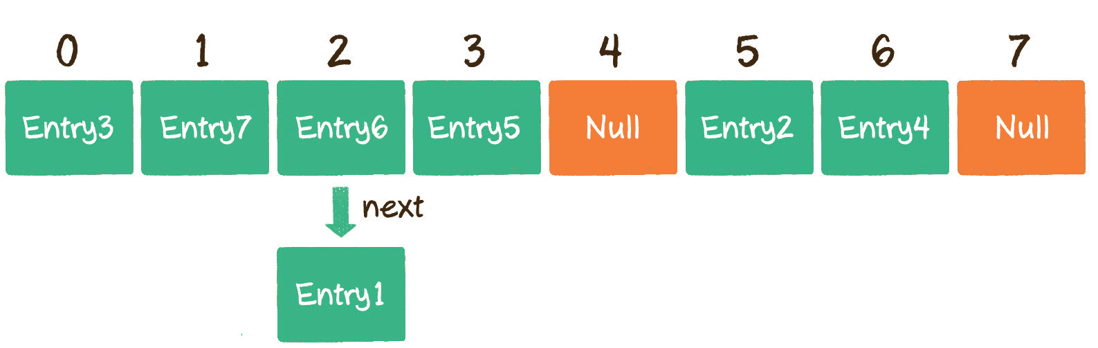
The open hash method, also known as the chain address method (zipper method), first uses the hash function to calculate the hash address of the key code set. The key codes with the same address belong to the same subset. Each subset is called a bucket. The elements in each bucket are linked through a single linked list, and the head nodes of each linked list are stored in the hash table. The zipper method is different from the open addressing method. Each element of the array in the zipper method is not only an Entry object, but also the head node of a linked list. Each Entry object points to its next Entry node through the next pointer. When the new Entry is mapped to the array position that conflicts with it, you only need to insert it into the corresponding linked list.
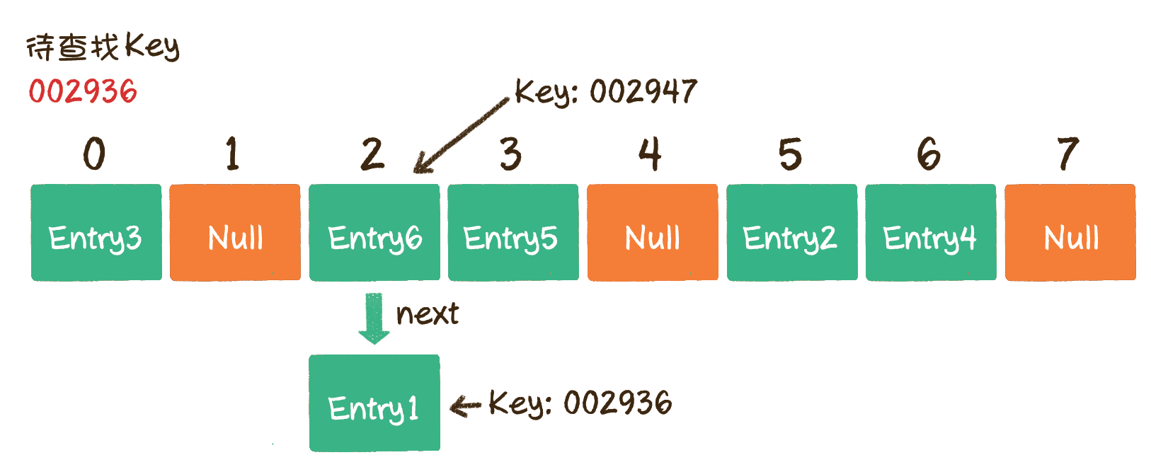
Let's look at how to find in zipper method:
Find the value corresponding to the Entry with Key 002936 in the hash table. What exactly should I do? Let's take the linked list method as an example. Step 1: convert Key into array subscript 2 through hash function. Step 2: find the element corresponding to array subscript 2. If the Key of this element is 002936, it will be found; It doesn't matter if the Key is not 002936. Since each element of the array corresponds to a linked list, we can slowly look down the linked list to see if we can find the node matching the Key.
Of course, hashing also needs to be expanded:
The number of buckets is certain. With the continuous insertion of elements, the number of elements in each bucket increases. In extreme cases, it may lead to a large number of linked list nodes in a bucket, which will affect the performance of the hash table. Therefore, under certain conditions, it is necessary to increase the capacity of the hash table. How can this condition be confirmed? The best case of hashing is that there is just one node hanging in each hash bucket. When you continue to insert elements, hash conflicts will occur every time. Therefore, when the number of elements is just equal to the number of buckets, you can add capacity to the hash table.
The steps of capacity expansion are as follows:
1. Expand the capacity and create a new empty Entry array, which is twice the length of the original array.
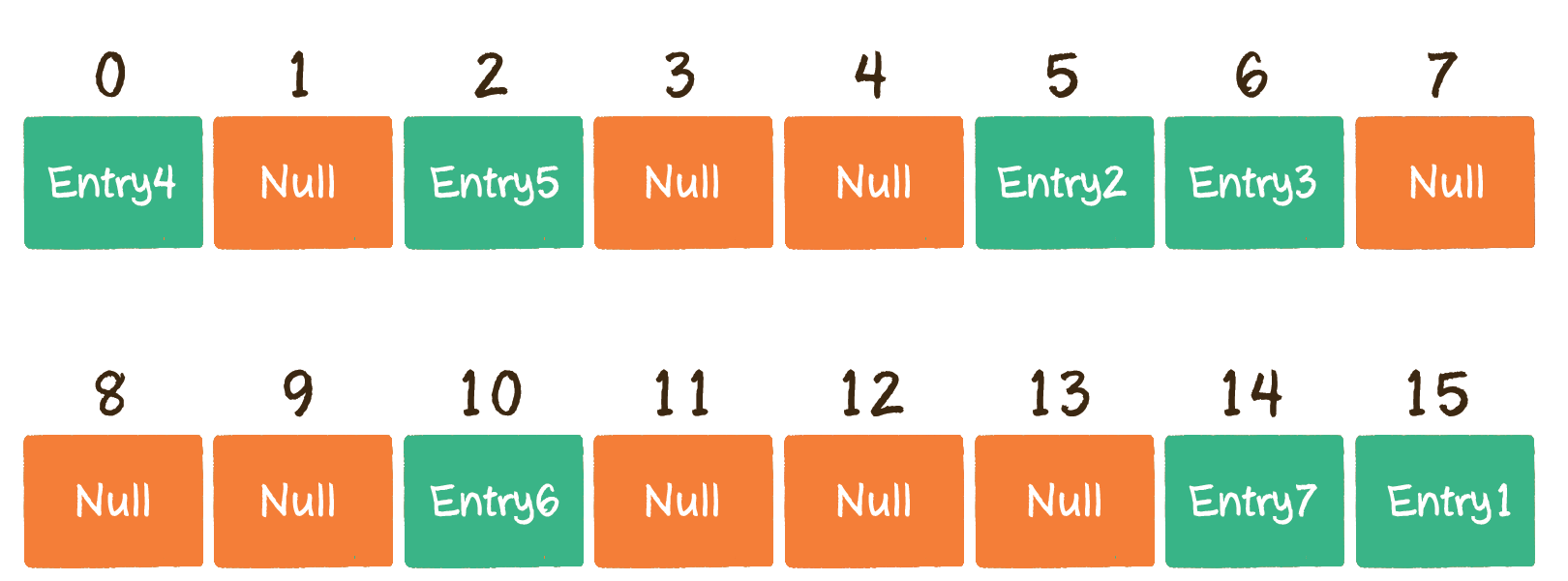
2. Re Hash, traverse the original Entry array, and re Hash all entries into the new array. Why re Hash? Because after the length is expanded, the rules of Hash also change. After capacity expansion, the originally crowded Hash table becomes sparse again, and the original entries are distributed as evenly as possible.
Before capacity expansion:
After capacity expansion:
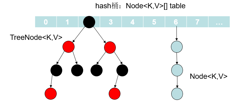
In the zipper method, if a chain conflicts very badly, you can choose to hang a red and black tree at the corresponding position.
For code
	template<class K>
		struct Hash
		{
			size_t operator()(const K& key)
			{
				return key;
			}
		};

		// Specialization
		template<>
		struct Hash < string >
		{
			// "int"  "insert"
			// The string is converted to a corresponding integer value, because the mapping position can be obtained only by integer
			// The expected - > string is different, and the transferred out integer value should be different as far as possible
			// "abcd" "bcad"
			// "abbb" "abca"
			size_t operator()(const string& s)
			{
				// BKDR Hash
				size_t value = 0;
				for (auto ch : s)
				{
					value += ch;
					value *= 131;
				}

				return value;
			}
		};

		template<class K, class V>
		struct HashNode
		{
			HashNode<K, V>* _next;
			pair<K, V> _kv;

			HashNode(const pair<K, V>& kv)
				:_next(nullptr)
				, _kv(kv)
			{}
		};

		template<class K, class V, class HashFunc = Hash<K>>
		class HashTable
		{
			typedef HashNode<K, V> Node;
		public:
			size_t GetNextPrime(size_t prime)
			{
				const int PRIMECOUNT = 28;
				static const size_t primeList[PRIMECOUNT] =
				{
					53ul, 97ul, 193ul, 389ul, 769ul,
					1543ul, 3079ul, 6151ul, 12289ul, 24593ul,
					49157ul, 98317ul, 196613ul, 393241ul, 786433ul,
					1572869ul, 3145739ul, 6291469ul, 12582917ul, 25165843ul,
					50331653ul, 100663319ul, 201326611ul, 402653189ul, 805306457ul,
					1610612741ul, 3221225473ul, 4294967291ul
				};

				size_t i = 0;
				for (; i < PRIMECOUNT; ++i)
				{
					if (primeList[i] > prime)
						return primeList[i];
				}

				return primeList[i];
			}

			bool Insert(const pair<K, V>& kv)
			{
				if (Find(kv.first))
					return false;

				HashFunc hf;
				// When the load factor reaches 1, increase the capacity
				if (_n == _table.size())
				{
					vector<Node*> newtable;
					//size_t newSize = _table.size() == 0 ? 8 : _table.size() * 2;
					//newtable.resize(newSize, nullptr);
					newtable.resize(GetNextPrime(_table.size()));

					// Traverse the nodes in the old table, recalculate the positions mapped to the new table, and hang them in the new table
					for (size_t i = 0; i < _table.size(); ++i)
					{
						if (_table[i])
						{
							Node* cur = _table[i];
							while (cur)
							{
								Node* next = cur->_next;
								size_t index = hf(cur->_kv.first) % newtable.size();
								// Head insert
								cur->_next = newtable[index];
								newtable[index] = cur;

								cur = next;
							}
							_table[i] = nullptr;
						}
					}

					_table.swap(newtable);
				}

				size_t index = hf(kv.first) % _table.size();
				Node* newnode = new Node(kv);

				// Head insert
				newnode->_next = _table[index];
				_table[index] = newnode;
				++_n;

				return true;
			}

			Node* Find(const K& key)
			{
				if (_table.size() == 0)
				{
					return false;
				}

				HashFunc hf;
				size_t index = hf(key) % _table.size();
				Node* cur = _table[index];
				while (cur)
				{
					if (cur->_kv.first == key)
					{
						return cur;
					}
					else
					{
						cur = cur->_next;
					}
				}

				return nullptr;
			}

			bool Erase(const K& key)
			{
				size_t index = hf(key) % _table.size();
				Node* prev = nullptr;
				Node* cur = _table[index];
				while (cur)
				{
					if (cur->_kv.first == key)
					{
						if (_table[index] == cur)
						{
							_table[index] = cur->_next;
						}
						else
						{
							prev->_next = cur->_next;
						}

						--_n;
						delete cur;
						return true;
					}

					prev = cur;
					cur = cur->_next;
				}

				return false;
			}

		private:
			vector<Node*> _table;
			size_t _n = 0;         // Number of valid data
		};