Deep learning, also known as "flower book". The book was written by three big men, Ian Goodfellow, Yoshua Bengio and Aaron Courville. It is a foundational classic textbook in the field of deep learning and is known as the "Bible" of deep learning.

The content of the original book is very rich, close to 800 pages. The content of this book is very deep and comprehensive, but the starting point is slightly higher and requires more basic knowledge of mathematical theory. Therefore, it is very helpful to summarize and summarize experience in time after reading. Shitoujun recently found a project on the summary of each chapter of the flower book on GitHub. The content is very concise. In addition to notes, some chapters are also equipped with codes, which is worthy of recommendation. Let's have a look.

The name of the project is deep learning book chapter summaries. The authors are Aman Dalmia and Ameya Godbole. The project address is:

https://github.com/dalmia/Deep-Learning-Book-Chapter-Summaries

primary coverage

The main chapters involved in the core notes of this flower book include:

• ch02 linear algebra
• ch03 probability and information theory
• ch04 numerical optimization
• ch07 deep learning regularization
• Optimization in ch08 depth model
• ch09 convolutional network
• ch11 practical methodology
• ch13 linear factor model

The form of notes is ipynb for easy opening and viewing on the Jupiter notebook. For example, let's take a look at the notes on linear algebra in Chapter 2.

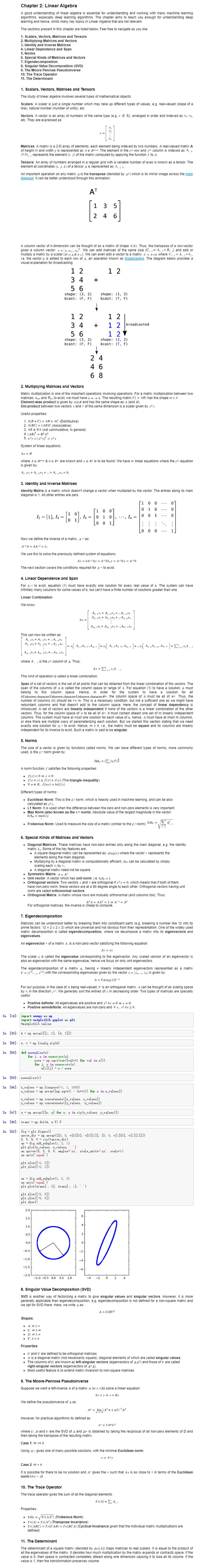
It can be seen that Jupyter's notes not only contain the summary of knowledge points, but also relevant codes. Let's look at the convolution network in Chapter 9, which is equipped with some complete image processing codes.

import numpy as np
from scipy import signal
from scipy import misc
import matplotlib.pyplot as plt

# %matplotlib inline

img = misc.ascent()
kernel = np.random.randn(5,5)
# kernel = np.array([[0,-10,0,10,0],[-10,-30,0,30,10],[0,-10,0,10,0]])

img = img.astype(np.float32)/255
orig_in = img

offsetx = offsety = 20
shift_in = np.zeros(orig_in.shape)
shift_in[offsetx:,offsety:] = img[:-offsetx,:-offsety]

rot_in = misc.imrotate(img, 90)
scale_in = misc.imresize(orig_in, 1.5)

output1 = signal.convolve2d(orig_in, kernel, mode='same')
output2 = signal.convolve2d(shift_in, kernel, mode='same')
output3 = signal.convolve2d(rot_in, kernel, mode='same')
output4 = signal.convolve2d(scale_in, kernel, mode='same')

fig, axes = plt.subplots(2, 4, figsize=(14, 7))
ax_orig = axes[0,0]
ax_shift = axes[0,1]
ax_rot = axes[0,2]
ax_scale = axes[0,3]

diff_orig = axes[1,0]
diff_shift = axes[1,1]
diff_rot = axes[1,2]
diff_scale = axes[1,3]

ax_orig.imshow(output1, cmap='gray')
ax_orig.set_title('Original')
ax_shift.imshow(output2, cmap='gray')
ax_shift.set_title('Shifted')
ax_rot.imshow(output3, cmap='gray')
ax_rot.set_title('Rotated')
ax_scale.imshow(output4, cmap='gray')
ax_scale.set_title('Scaled')

def shift(arr, offset):
    output = np.zeros(arr.shape)
    output[offset:, offset:] = arr[:-offset,:-offset]
    return output

def rotate(arr, angle):
    return misc.imrotate(arr, angle)

def resize(arr, scale):
    return misc.imresize(arr, scale)

diff_orig.hist(np.ravel(output1),bins=100)
diff_orig.set_title('Output histogram')
diff_shift.hist(np.ravel(np.abs(output2-shift(output1, 20))),bins=100)
diff_shift.set_title('Shift histogram difference')
diff_rot.hist(np.ravel(np.abs(output3-rotate(output1, 10))),bins=100)
diff_rot.set_title('Rotate histogram difference')
diff_scale.hist(np.ravel(np.abs(output4-resize(output1, 1.5))),bins=100)
diff_scale.set_title('Scale histogram difference')

ax_orig.set_xticks([])
ax_shift.set_xticks([])
ax_rot.set_xticks([])
ax_scale.set_xticks([])

ax_orig.set_yticks([])
ax_shift.set_yticks([])
ax_rot.set_yticks([])
ax_scale.set_yticks([])

plt.tight_layout()
# plt.show()
plt.savefig('images/conv_equivariance.png')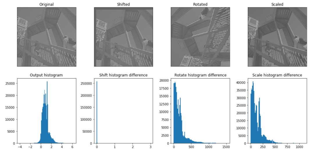

Code example for pooling layer:

import numpy as np
np.random.seed(101)

from scipy import signal
from scipy import misc
import matplotlib.pyplot as plt
%matplotlib inline

img = misc.ascent()
img = img.astype(np.float32)/255

# The image is more interesting here
orig_in = img[-200:,-300:-100]
offsetx = offsety = 15
shift_in = img[-200-offsetx:-offsetx,-300-offsety:-100-offsety]
kernel1 = np.random.randn(5,5)
kernel2 = np.random.randn(5,5)
kernel3 = np.random.randn(5,5)

def sigmoid(arr):
    # Lazy implementation of sigmoid activation
    return 1./(1 + np.exp(-arr))

def maxpool(arr, poolsize, stride):
    # Lazy looping implementation of maxpool
    output_shape = np.floor((np.array(arr.shape)-poolsize)/stride)+1
    output_shape = output_shape.astype(np.int32)
    output = np.zeros(output_shape)
    for x in range(output_shape[0]):
        for y in range(output_shape[1]):
            output[x,y] = np.max(arr[x*stride:x*stride+poolsize,y*stride:y*stride+poolsize])
    return output

output1_1 = signal.convolve2d(orig_in, kernel1, mode='valid')
pool1_1 = maxpool(output1_1, 2, 2)
actv1_1 = sigmoid(pool1_1)
output1_2 = signal.convolve2d(actv1_1, kernel2, mode='valid')
pool1_2 = maxpool(output1_2, 2, 2)
actv1_2 = sigmoid(pool1_2)
output1_3 = signal.convolve2d(actv1_2, kernel3, mode='valid')
pool1_3 = maxpool(output1_3, 2, 2)

output2_1 = signal.convolve2d(shift_in, kernel1, mode='valid')
pool2_1 = maxpool(output2_1, 2, 2)
actv2_1 = sigmoid(pool2_1)
output2_2 = signal.convolve2d(actv2_1, kernel2, mode='valid')
pool2_2 = maxpool(output2_2, 2, 2)
actv2_2 = sigmoid(pool2_2)
output2_3 = signal.convolve2d(actv2_2, kernel3, mode='valid')
pool2_3 = maxpool(output2_3, 2, 2)

fig, axes = plt.subplots(4, 3, figsize=(10, 10))

k1, k2, k3 = axes[0,:]
p1_1, p1_2, p1_3 = axes[1,:]
p2_1, p2_2, p2_3 = axes[2,:]
h1, h2, h3 = axes[3,:]

k1.imshow(kernel1, cmap='gray')
k1.set_title('kernel1')
k2.imshow(kernel2, cmap='gray')
k2.set_title('kernel2')
k3.imshow(kernel3, cmap='gray')
k3.set_title('kernel3')
k1.set_xticks([])
k2.set_xticks([])
k3.set_xticks([])
k1.set_yticks([])
k2.set_yticks([])
k3.set_yticks([])

p1_1.imshow(pool1_1, cmap='gray')
p1_1.set_title('pool1_1')
p1_2.imshow(pool1_2, cmap='gray')
p1_2.set_title('pool1_2')
p1_3.imshow(pool1_3, cmap='gray')
p1_3.set_title('pool1_3')
p1_1.set_xticks([])
p1_2.set_xticks([])
p1_3.set_xticks([])
p1_1.set_yticks([])
p1_2.set_yticks([])
p1_3.set_yticks([])

p2_1.imshow(pool2_1, cmap='gray')
p2_1.set_title('pool2_1')
p2_2.imshow(pool2_2, cmap='gray')
p2_2.set_title('pool2_2')
p2_3.imshow(pool2_3, cmap='gray')
p2_3.set_title('pool2_3')
p2_1.set_xticks([])
p2_2.set_xticks([])
p2_3.set_xticks([])
p2_1.set_yticks([])
p2_2.set_yticks([])
p2_3.set_yticks([])

h1.hist(np.ravel(np.abs(pool1_1-pool2_1)),bins=100)
h1.set_title('Pool 1 diff')
h2.hist(np.ravel(np.abs(pool1_2-pool2_2)),bins=100)
h2.set_title('Pool 2 diff')
h3.hist(np.ravel(np.abs(pool1_3-pool2_3)),bins=100)
h3.set_title('Pool 3 diff')

plt.tight_layout()
# plt.show()
plt.savefig('images/pool_invariance.png')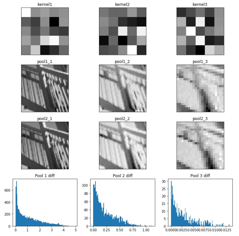

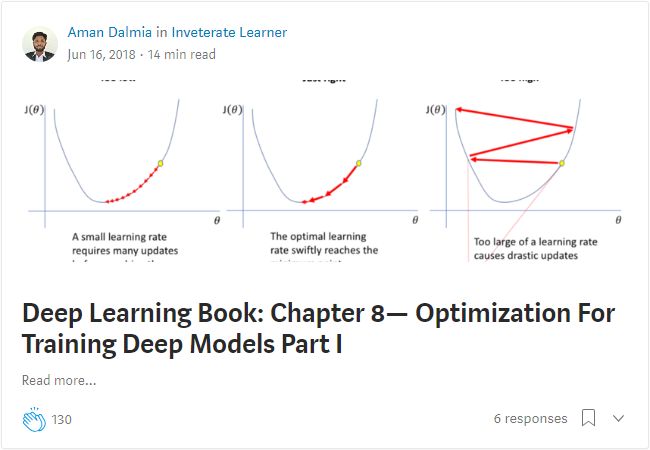
Blog notes

The author of the project also published the refined notes of Huashu on his personal website at:

https://medium.com/inveterate-learner/tagged/deep-learning

Additional resources

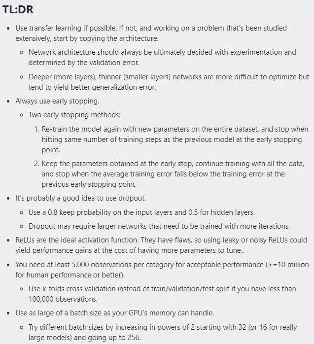
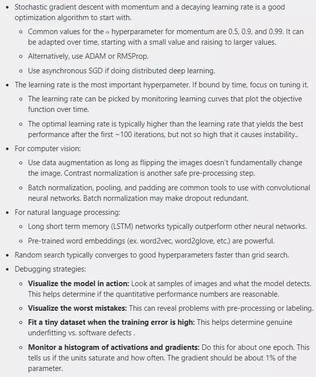
In addition to the summary of the key chapters of the flower book, shitoujun also recommends a rule of thumb on the flower book summarized by Jeff Macaluso, a Microsoft computer software engineer!

Online reading address:

https://jeffmacaluso.github.io/post/DeepLearningRulesOfThumb/

Offline address

Link:

https://pan.baidu.com/s/1eLlJy3xB6Hs0w_Q7bO536g

Extraction code: 7q1d