Our community has new technology sharing partners 🎉🎉🎉
a warm welcome 👏
As a qualified Porter, I must do something to express my joy: Handling ~ handling ~ immediate handling ~
Article source| Hengyuan cloud community
Original address| New hybrid Transformer module (MTM)
Original author Dong Dong
abstract
| Existing problems | Although U-Net has achieved great success in medical image segmentation, it lacks the ability to explicitly model long-term dependencies. Visual Transformer has become an alternative segmentation structure in recent years because of its inherent ability to capture long-range correlation through self attention (SA). |
|---|---|
| Existing problems | However, Transformer usually relies on large-scale pre training and has high computational complexity. In addition, SA can only model self affinities in a single sample, ignoring the potential correlation of the whole data set |
| Thesis method | A new hybrid Transformer module (MTM) is proposed for simultaneous inter affinities learning and intra affinities learning. MTM first effectively calculates the internal affinities of the window through local global Gaussian weighted self attention (LGG-SA). Then, pay attention to mining the relationship between data samples through external. Using MTM algorithm, a MT UNET model for medical image segmentation is constructed |
Method

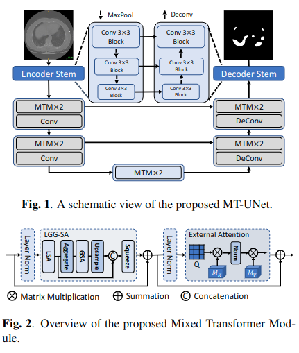
As shown in Figure 1. The network is based on encoder decoder structure
- In order to reduce the computational cost, MTMs is only used for deep layers with small space,
- The classical convolution operation is still used in shallow layer. This is because the shallow layer mainly focuses on local information and contains more high-resolution details.
MTM
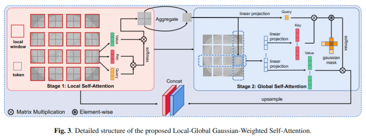
As shown in Figure 2. MTM is mainly composed of LGG-SA and EA.
LGG-SA is used to model short-term and long-term dependencies with different granularity, while EA is used to mine the correlation between samples.
This module is to replace the original Transformer encoder to improve its performance in visual tasks and reduce the time complexity
LGG-SA(Local-Global Gaussian-Weighted Self-Attention)
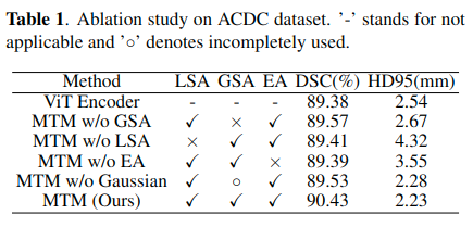
The traditional SA module gives the same attention to all tokens, while lgg-sa is different. It can focus more on the adjacent area by using local global self attention and Gaussian mask. Experiments show that this method can improve the performance of the model and save computing resources. The detailed design of the module is shown in Figure 3
Local global self attention
In computer vision, the correlation between adjacent regions is often more important than that between distant regions. When calculating the attention map, it does not need to pay the same price for the farther regions.
Therefore, local global self attention is proposed.
- Each local window in stage1 above contains four token s. local SA calculates the internal affinities in each window.
- The tokens in each window are aggregated into a global token by aggregate, which represents the main information of the window. For aggregate functions, lightweight dynamic convolution (ldconv) has the best performance.
- After obtaining the entire feature map of down sampling, global SA can be executed with less overhead (stage2 above).

Where \ (X \in R^{H \times W \times C} \)
The self attention codes of local windows in stage1 are as follows:
class WinAttention(nn.Module):
    def __init__(self, configs, dim):
        super(WinAttention, self).__init__()
        self.window_size = configs["win_size"]
        self.attention = Attention(dim, configs)

    def forward(self, x):
        b, n, c = x.shape
        h, w = int(np.sqrt(n)), int(np.sqrt(n))
        x = x.permute(0, 2, 1).contiguous().view(b, c, h, w)
        if h % self.window_size != 0:
            right_size = h + self.window_size - h % self.window_size
            new_x = torch.zeros((b, c, right_size, right_size))
            new_x[:, :, 0:x.shape[2], 0:x.shape[3]] = x[:]
            new_x[:, :, x.shape[2]:,
                  x.shape[3]:] = x[:, :, (x.shape[2] - right_size):,
                                   (x.shape[3] - right_size):]
            x = new_x
            b, c, h, w = x.shape
        x = x.view(b, c, h // self.window_size, self.window_size,
                   w // self.window_size, self.window_size)
        x = x.permute(0, 2, 4, 3, 5,
                      1).contiguous().view(b, h // self.window_size,
                                           w // self.window_size,
                                           self.window_size * self.window_size,
                                           c).cuda()
        x = self.attention(x)  #  (b, p, p, win, c) calculate the self attention of tokens in the local window
        return x
The aggregate function code is as follows
class DlightConv(nn.Module):
    def __init__(self, dim, configs):
        super(DlightConv, self).__init__()
        self.linear = nn.Linear(dim, configs["win_size"] * configs["win_size"])
        self.softmax = nn.Softmax(dim=-1)

    def forward(self, x):  # (b, p, p, win, c)
        h = x
        avg_x = torch.mean(x, dim=-2)  # (b, p, p, c)
        x_prob = self.softmax(self.linear(avg_x))  # (b, p, p, win)

        x = torch.mul(h,
                      x_prob.unsqueeze(-1))  # (b, p, p, win, c)
        x = torch.sum(x, dim=-2)  # (b, p, p, c)
        return x
Gaussian-Weighted Axial Attention
Different from the LSA using the original SA, a Gaussian weighted axial attention (GWAA) method is proposed. GWAA enhances the perceptual full weight of adjacent regions through a learnable Gaussian matrix, and reduces the time complexity due to axial attention.
- In the figure above, the features in the third row and the third column of the feature map in stage2 are obtained by linear projection \ (q_{i, j} \)
- Perform linear projection on all the features of the row and column of the feature point to obtain \ (K_{i, j} \)
And \ (V {I, J} \) - The Euclidean distance between the feature point and all K and V is defined as \ (D {I, J} \)
The final Gaussian weighted axial attention output is
And simplified to
The axial attention code is as follows:
class Attention(nn.Module):
    def __init__(self, dim, configs, axial=False):
        super(Attention, self).__init__()
        self.axial = axial
        self.dim = dim
        self.num_head = configs["head"]
        self.attention_head_size = int(self.dim / configs["head"])
        self.all_head_size = self.num_head * self.attention_head_size

        self.query_layer = nn.Linear(self.dim, self.all_head_size)
        self.key_layer = nn.Linear(self.dim, self.all_head_size)
        self.value_layer = nn.Linear(self.dim, self.all_head_size)

        self.out = nn.Linear(self.dim, self.dim)
        self.softmax = nn.Softmax(dim=-1)

    def transpose_for_scores(self, x):
        new_x_shape = x.size()[:-1] + (self.num_head, self.attention_head_size)
        x = x.view(*new_x_shape)
        return x

    def forward(self, x):
        # first row and col attention
        if self.axial:
             # x: (b, p, p, c)
            # row attention (single head attention)
            b, h, w, c = x.shape
            mixed_query_layer = self.query_layer(x)
            mixed_key_layer = self.key_layer(x)
            mixed_value_layer = self.value_layer(x)

            query_layer_x = mixed_query_layer.view(b * h, w, -1)
            key_layer_x = mixed_key_layer.view(b * h, w, -1).transpose(-1, -2)  # (b*h, -1, w)
            attention_scores_x = torch.matmul(query_layer_x,
                                              key_layer_x)  # (b*h, w, w)
            attention_scores_x = attention_scores_x.view(b, -1, w,
                                                         w)  # (b, h, w, w)

            # col attention  (single head attention)
            query_layer_y = mixed_query_layer.permute(0, 2, 1,
                                                      3).contiguous().view(
                                                          b * w, h, -1)
            key_layer_y = mixed_key_layer.permute(
                0, 2, 1, 3).contiguous().view(b * w, h, -1).transpose(-1, -2)  # (b*w, -1, h)
            attention_scores_y = torch.matmul(query_layer_y,
                                              key_layer_y)  # (b*w, h, h)
            attention_scores_y = attention_scores_y.view(b, -1, h,
                                                         h)  # (b, w, h, h)

            return attention_scores_x, attention_scores_y, mixed_value_layer

        else:

            mixed_query_layer = self.query_layer(x)
            mixed_key_layer = self.key_layer(x)
            mixed_value_layer = self.value_layer(x)

            query_layer = self.transpose_for_scores(mixed_query_layer).permute(
                0, 1, 2, 4, 3, 5).contiguous()  # (b, p, p, head, n, c)
            key_layer = self.transpose_for_scores(mixed_key_layer).permute(
                0, 1, 2, 4, 3, 5).contiguous()
            value_layer = self.transpose_for_scores(mixed_value_layer).permute(
                0, 1, 2, 4, 3, 5).contiguous()

            attention_scores = torch.matmul(query_layer,
                                            key_layer.transpose(-1, -2))
            attention_scores = attention_scores / math.sqrt(
                self.attention_head_size)
            atten_probs = self.softmax(attention_scores)

            context_layer = torch.matmul(
                atten_probs, value_layer)  # (b, p, p, head, win, h)
            context_layer = context_layer.permute(0, 1, 2, 4, 3,
                                                  5).contiguous()
            new_context_layer_shape = context_layer.size()[:-2] + (
                self.all_head_size, )
            context_layer = context_layer.view(*new_context_layer_shape)
            attention_output = self.out(context_layer)

        return attention_output
The Gaussian weighting code is as follows:
class GaussianTrans(nn.Module):
    def __init__(self):
        super(GaussianTrans, self).__init__()
        self.bias = nn.Parameter(-torch.abs(torch.randn(1)))
        self.shift = nn.Parameter(torch.abs(torch.randn(1)))
        self.softmax = nn.Softmax(dim=-1)

    def forward(self, x):
        x, atten_x_full, atten_y_full, value_full = x  #x(b, h, w, c) atten_x_full(b, h, w, w)   atten_y_full(b, w, h, h) value_full(b, h, w, c)
        new_value_full = torch.zeros_like(value_full)

        for r in range(x.shape[1]):  # row
            for c in range(x.shape[2]):  # col
                atten_x = atten_x_full[:, r, c, :]  # (b, w)
                atten_y = atten_y_full[:, c, r, :]  # (b, h)

                dis_x = torch.tensor([(h - c)**2 for h in range(x.shape[2])
                                      ]).cuda()  # (b, w)
                dis_y = torch.tensor([(w - r)**2 for w in range(x.shape[1])
                                      ]).cuda()  # (b, h)

                dis_x = -(self.shift * dis_x + self.bias).cuda()
                dis_y = -(self.shift * dis_y + self.bias).cuda()

                atten_x = self.softmax(dis_x + atten_x)
                atten_y = self.softmax(dis_y + atten_y)

                new_value_full[:, r, c, :] = torch.sum(
                    atten_x.unsqueeze(dim=-1) * value_full[:, r, :, :] +
                    atten_y.unsqueeze(dim=-1) * value_full[:, :, c, :],
                    dim=-2)
        return new_value_full
The complete code of local global self attention is as follows:
class CSAttention(nn.Module):
    def __init__(self, dim, configs):
        super(CSAttention, self).__init__()
        self.win_atten = WinAttention(configs, dim)
        self.dlightconv = DlightConv(dim, configs)
        self.global_atten = Attention(dim, configs, axial=True)
        self.gaussiantrans = GaussianTrans()
        #self.conv = nn.Conv2d(dim, dim, 3, padding=1)
        #self.maxpool = nn.MaxPool2d(2)
        self.up = nn.UpsamplingBilinear2d(scale_factor=4)
        self.queeze = nn.Conv2d(2 * dim, dim, 1)

    def forward(self, x):
        '''
        :param x: size(b, n, c)
        :return:
        '''
        origin_size = x.shape
        _, origin_h, origin_w, _ = origin_size[0], int(np.sqrt(
            origin_size[1])), int(np.sqrt(origin_size[1])), origin_size[2]
        x = self.win_atten(x)  # (b, p, p, win, c)
        b, p, p, win, c = x.shape
        h = x.view(b, p, p, int(np.sqrt(win)), int(np.sqrt(win)),
                   c).permute(0, 1, 3, 2, 4, 5).contiguous()
        h = h.view(b, p * int(np.sqrt(win)), p * int(np.sqrt(win)),
                   c).permute(0, 3, 1, 2).contiguous()  # (b, c, h, w)

        x = self.dlightconv(x)  # (b, p, p, c)
        atten_x, atten_y, mixed_value = self.global_atten(
            x)  # (b, h, w, w) (b, w, h, h) (b, h, w, c) here h, W is p
        gaussian_input = (x, atten_x, atten_y, mixed_value)
        x = self.gaussiantrans(gaussian_input)  # (b, h, w, c)
        x = x.permute(0, 3, 1, 2).contiguous()  # (b, c, h, w)

        x = self.up(x)
        x = self.queeze(torch.cat((x, h), dim=1)).permute(0, 2, 3,
                                                          1).contiguous()
        x = x[:, :origin_h, :origin_w, :].contiguous()
        x = x.view(b, -1, c)

        return x
EA
External attention (EA) is used to solve the problem that SA cannot use the relationship between different input data samples.
Different from using each sample's own linear transformation to calculate the self attention of attention score, in EA, all data samples share two memory units MK and MV (as shown in Figure 2), which describe the most important information of the whole data set.
EA code is as follows:
class MEAttention(nn.Module):
    def __init__(self, dim, configs):
        super(MEAttention, self).__init__()
        self.num_heads = configs["head"]
        self.coef = 4
        self.query_liner = nn.Linear(dim, dim * self.coef)
        self.num_heads = self.coef * self.num_heads
        self.k = 256 // self.coef
        self.linear_0 = nn.Linear(dim * self.coef // self.num_heads, self.k)
        self.linear_1 = nn.Linear(self.k, dim * self.coef // self.num_heads)

        self.proj = nn.Linear(dim * self.coef, dim)

    def forward(self, x):
        B, N, C = x.shape
        x = self.query_liner(x)  # (b, n, 4c)
        x = x.view(B, N, self.num_heads, -1).permute(0, 2, 1,
                                                     3)  #  (b, h, n, 4c/h)

        attn = self.linear_0(x)  # (b, h, n, 256/4)

        attn = attn.softmax(dim=-2)  # (b, h, 256/4)
        attn = attn / (1e-9 + attn.sum(dim=-1, keepdim=True))  # (b, h, 256/4)

        x = self.linear_1(attn).permute(0, 2, 1, 3).reshape(B, N, -1)

        x = self.proj(x)

        return x
EXPERIMENTS


