Preface

The climbing method is an optimization algorithm. It generally starts from a random point, then calculates the function value of each point step by step until an optimal solution (local optimal) is found, so it is a local search algorithm, which means it is suitable for single peak optimization problems or after global optimization algorithm is applied.

There are three shortcomings of the climbing method:
(1) Local optimum: The nature of the algorithm determines that it is very easy to fall into local optimum and difficult to jump out;
(2) Flat roof:
Flat roof is an area in the state space where the value of the evaluation function is essentially unchanged and F(x) is constant around a local point. Once the search has reached a flat top, the search cannot determine the best direction to search, resulting in random walks, which makes the search less efficient.
(3) Ridges:
Ridges may have steep slopes, so the search can reach the top of the ridge more easily, but the top of the ridge may tilt very gently between the peaks and the search will make little progress.

To get a better solution to the above problems, the traditional practice is to use the hill-climbing algorithm many times (starting from different initial solutions) to find the best solution from multiple local optimal solutions, which may be the global optimal solution.

This paper improves the classical hill-climbing algorithm so that it does not need to produce multiple random initial solutions to "climb" a mountain, but only "climb" once to find the highest mountain.

Tip: The following is the main body of this article. The following cases can be used as reference.

1. Hill-climbing algorithm

The hill-climbing algorithm simulates the process of climbing, randomly selecting a location to climb a mountain, moving in a higher direction each time until the top is reached, that is, selecting the optimal solution in the adjacent space each time as the current solution until the local optimal solution is reached. Thus, the algorithm will fall into the local optimal solution, and whether or not the global optimal solution can be obtained depends on the location of the initial point. If the initial point is selected as the global optimal solution Near the solution, the global optimal solution may be obtained.
Algorithmic description:
Start with the current node and compare with the values of neighboring nodes around it. If the current node is the largest, then the current node is returned as the maximum (that is, the highest point of the mountain); Conversely, replace the current node with the highest neighbor node to achieve the goal of climbing to the height of the mountain. Loop like this until you reach the highest point.

Algorithmic implementation:
Late Update >>

2. Algorithm Improvement - Detector

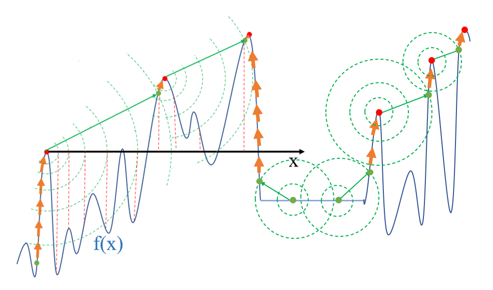
This is a comparison of the classic hill-climbing algorithm to randomly placing m ants at random points on a mountain. Ants choose whether to go forward or not based on the height (x*) of the point within L unit length of the current position (x*). If the current position (x*) is the center of the circle, the height F(x*+L) of each point on the radius is less than the height F (x*) of the current point (x*). The location is considered optimal (local) and the ants do not move. Otherwise, the ant continues to advance to the next higher point until it is no higher. After such a climb, m ants will find a highest point (local), that is, a total of M highest points (local), the maximum of which may be the global optimal value (the more ants there are, the greater the probability of finding the global optimal value).

This paper improves the traditional hill-climbing algorithm so that it can find the global optimal value at once, and the algorithm will not sink into the plain (the height f(x) is a constant in the field of a point (x^).
Algorithmic description:
First, the ants are empowered: the ants have detector functions (like radar); and the ants fly.
Step 1: On the basis of the classical climbing algorithm, the ant climbs to the top of the mountain (local optimal value):
Step 2: Detect if there is a higher point in the distance than the current position, if there is, fly to a higher position, and proceed with Step 1. If not, this point is the global optimal value.
Similarly for plain problems, when the ants are on a flat surface, detect if there are any higher points around them. If there are, climb to the first higher point and proceed step one and step two until they reach the highest point.
Schematic algorithm:

1. Recursively find the local optimal value

The climbing code is as follows (example):

def cycle(i,r,R2,T2):
   if(i>=5 or i<=-5):
      if(i>5):
         obj.append(i-r)
         ax2.scatter(i-r,fun(i-r))
         return
      if(i<-5):
         obj.append(i+r)
         ax2.scatter(i+r,fun(i+r))
         return  #Exit cycle beyond defined field
   y_i=fun(i)
   ax1.scatter(i,y_i)
   plt.pause(0.02)
   if(fun(i+r)<=y_i and fun(i-r)<=y_i):
      radiation(i,r,R2,T2)
##      ax1.scatter(i,fun(i))
   elif(fun(i+r)<y_i and fun(i-r)>=y_i):
##      r=abs(r+0.02)
      cycle(i-r,r,R2,T2)#Find the optimal value from the negative x-axis direction

   elif(fun(i+r)>=y_i and fun(i-r)<y_i):
##      r+=0.02#Finding the Optimal Value Forward from the x-axis
      cycle(i+r,r,R2,T2)
   else: #Bidirectional detection if the current point is at the bottom of a valley  
      cycle(i+r,r,R2,T2)
      cycle(i-r,r,R2,T2)#Find the optimal value from the negative x-axis direction
   return  

2. Detector Search for Global Optimum

The code is as follows (example):

def radiation(i,R1,R2,T2):# Telescope Function, i Current Locally Optimal Location R: Radiation Radius, T: Number of Emissions
   y_i=fun(i)
   t_2=0
   r2=R2
   i_r=i+r2
   i_l=i-r2
   while True:
      if(i_r>5 or i_l<-5):
         obj.append(i)
         ax2.scatter(i,fun(i))
         break
      if t_2==T2 :
         obj.append(i)
         ax2.scatter(i,fun(i))
         break
      y_f=fun(i_r)
      y_b=fun(i_l)
      if(y_f>y_i and y_b>y_i):
         cycle(i_r,R1,R2,T2)
         cycle(i_l,R1,R2,T2)
         break
      elif(y_f>y_i and y_b<y_i):
         cycle(i_r,R1,R2,T2)
         break
      elif(y_f<y_i and y_b>y_i):
         cycle(i_l,R1,R2,T2)
         break
      else:
         t_2=t_2+1
         i_r=i_r+r2
         i_l=i_l-r2
   return

Call the improved algorithm to find the optimal value.

def rad_cyc(R_1,R_2,T_1,T_2,*objection):
   t_1=0
   while (t_1<T_1):
      point=round(np.random.uniform(-5,5),5)
      r=R_1
      cycle(point,r,R_2,T_2)
      t_1+=1
   print(obj)
   ax2.text(2,2,'number:%d'%len(obj))
   plt.show()
rad_cyc(0.05,0.1,5,30,obj)

Run result:

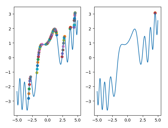
The left image shows the ants'forward path point, and the right image shows the final location. Because the code has an unknown BUG, sometimes the result will fall into local optimum, I have limited level and am working on >>>
Full code:

import numpy as np
import matplotlib.pyplot as plt
x=np.arange(-5,5,0.01)
y=[]
obj=[]#Used to store local optimum values
y=np.cos(x)+0.5*x+np.sin(x**2)
def fun(x):##objective function
   return np.cos(x)+0.5*x+np.sin(x**2)
f=plt.figure()
ax1=plt.subplot(1,2,1)
ax2=plt.subplot(1,2,2)
ax1.plot(x,y)
ax2.plot(x,y)

def radiation(i,R1,R2,T2):# Telescope Function, i Current Locally Optimal Location R: Radiation Radius, T: Number of Emissions
   y_i=fun(i)
   t_2=0
   r2=R2
   i_r=i+r2
   i_l=i-r2
   while True:
      if(i_r>5 or i_l<-5):
         obj.append(i)
         ax2.scatter(i,fun(i))
         break
      if t_2==T2 :
         obj.append(i)
         ax2.scatter(i,fun(i))
         break
      y_f=fun(i_r)
      y_b=fun(i_l)
      if(y_f>y_i and y_b>y_i):
         cycle(i_r,R1,R2,T2)
         cycle(i_l,R1,R2,T2)
         break
      elif(y_f>y_i and y_b<y_i):
         cycle(i_r,R1,R2,T2)
         break
      elif(y_f<y_i and y_b>y_i):
         cycle(i_l,R1,R2,T2)
         break
      else:
         t_2=t_2+1
         i_r=i_r+r2
         i_l=i_l-r2
   return
def cycle(i,r,R2,T2):
   if(i>=5 or i<=-5):
      if(i>5):
         obj.append(i-r)
         ax2.scatter(i-r,fun(i-r))
         return
      if(i<-5):
         obj.append(i+r)
         ax2.scatter(i+r,fun(i+r))
         return  #Exit cycle beyond defined field
   y_i=fun(i)
   ax1.scatter(i,y_i)
   plt.pause(0.02)
   if(fun(i+r)<=y_i and fun(i-r)<=y_i):
      radiation(i,r,R2,T2)
##      ax1.scatter(i,fun(i))
   elif(fun(i+r)<y_i and fun(i-r)>=y_i):
##      r=abs(r+0.02)#Detection step, increasing step by step
      cycle(i-r,r,R2,T2)#Find the optimal value from the negative x-axis direction

   elif(fun(i+r)>=y_i and fun(i-r)<y_i):
##      r+=0.02#Finding the Optimal Value Forward from the x-axis
      cycle(i+r,r,R2,T2)
   else: #If the detector is at the bottom of the valley, two-way detection  
      cycle(i+r,r,R2,T2)
      cycle(i-r,r,R2,T2)#Find the optimal value from the negative x-axis direction
   return  
def rad_cyc(R_1,R_2,T_1,T_2,*objection):
   t_1=0
   while (t_1<T_1):#Set the number of iterations, that is, the number of detectors
      point=round(np.random.uniform(-5,5),5)
      r=R_1#Detect Half-kilogram Return Value
      cycle(point,r,R_2,T_2)
      t_1+=1
   print(obj)
   ax2.text(2,2,'number:%d'%len(obj))
   plt.show()
rad_cyc(0.05,0.1,5,30,obj)

For plains, an additional objective function is set:

def fun(x):
   if(x>=-5 and x<-1):return -(x+2)**2+2
   elif(x>=-1 and x<=1):return 1
   else: return -2*(x-2)**2+3

Run result:

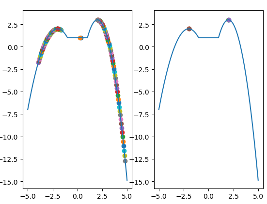
Code has bugs, is being processed, and will be updated >> when resolved

summary

This improved hill-climbing algorithm can effectively avoid falling into local optimum and plain. For the problem of slow ridge iteration speed, variable step can be used instead of constant step to increase iteration speed. Reference resources:

1.python hill-climbing algorithm
2.Python Implements Random Hill Climb Algorithms
3.Hill climbing algorithm
4.Random optimization algorithm-hill climbing VS simulated annealing