Overfitting and Unfitting

Over-fitting phenomenon: The performance of the model in leaving validation data always reaches its peak after several rounds, and then begins to decline.
Unfitting phenomenon: The less the loss of training data, the less the loss of testing data.

Concepts of optimization and generalization

Optimizing: Adjusting the model to get the best performance on training data
Generalization: It refers to the performance of trained models on unprecedented data. The purpose of machine learning is, of course, to get good generalization.

How to Solve the Problem of Overfitting

• The best solution is to get more training data.
• The sub-optimal solution is regularization: adjusting the amount of information that the model allows to store (constraining the amount of information that the model allows to store)

The main regularization methods are:

• Reduce network size
• Adding Weight Regularization
• Add dropout regularization

Reduce network size

The simplest way to prevent over-fitting is to reduce the size of the model, that is, to reduce the number of learnable parameters in the model (which is determined by the number of layers and the number of units in each layer). In fact, the principle of this method is to reduce the capacity of parameters.
Why is this possible?
For example, a model with 500,000 binary parameters can easily learn the categories corresponding to all the digits in the MNIST training set - we only need 50,000 digits each corresponding to 10 binary parameters. But this model is useless for the classification of new digital samples. There is no good generalization for new data.

Here's what you need to understand: * Deep learning models are usually good at fitting training data, but the real challenge is generalization, not fitting.

There is no standard formula for determining the size of a network: determining the optimal number of layers or the optimal size of each layer. Usually through the test: from small to large test parameters. Finally, determine a size.

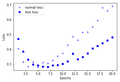
The following cases: It can be seen intuitively that smaller networks begin to over-fit later than larger networks, and larger networks over-fit more seriously. The fluctuation of verification loss is also greater.

from keras.datasets import imdb

(train_data,train_labels),(test_data,test_labels) = imdb.load_data(num_words=10000)
# Encoding an integer sequence into a binary matrix
import numpy as np

def vectorize_sequences(sequences,dimension=10000):
    results = np.zeros((len(sequences),dimension))
    for i,sequence in enumerate(sequences):
        results[i,sequence] = 1.
    return results

# Transform data into matrices
x_train = vectorize_sequences(train_data)
x_test = vectorize_sequences(test_data)

# Vectorization of labels
y_train = np.asarray(train_labels).astype('float32')
y_test = np.asarray(test_labels).astype('float32')

from keras import models
from keras import layers

model = models.Sequential()
model.add(layers.Dense(16, activation='relu',input_shape=(10000,)))
model.add(layers.Dense(16, activation='relu'))
model.add(layers.Dense(1,activation='sigmoid'))

# Standard optimizer
model.compile(optimizer='rmsprop',
              loss = 'binary_crossentropy',
              metrics = ['accuracy']) # Monitoring accuracy in training process

# Fabrication of Verification Set
x_val = x_train[:10000]
partial_x_train = x_train[10000:]

y_val = y_train[:10000]
partial_y_train = y_train[10000:]

history = model.fit(partial_x_train,
                   partial_y_train,
                   epochs=20,
                   batch_size=512,
                   validation_data=(x_val,y_val))

history_dict = history.history

from keras import models
from keras import layers

model2 = models.Sequential()
model2.add(layers.Dense(4, activation='relu',input_shape=(10000,)))
model2.add(layers.Dense(4, activation='relu'))
model2.add(layers.Dense(1,activation='sigmoid'))

# Standard optimizer
model2.compile(optimizer='rmsprop',
              loss = 'binary_crossentropy',
              metrics = ['accuracy']) # Monitoring accuracy in training process

history2 = model2.fit(partial_x_train,
                   partial_y_train,
                   epochs=20,
                   batch_size=512,
                   validation_data=(x_val,y_val))

history_dict2 = history2.history

# Drawing training loss congratulations to verify loss
import matplotlib.pyplot as plt

history_dict = history.history
loss_values_normal = history_dict['val_loss']
loss_values_less = history_dict2['val_loss']

epochs = range(1,len(loss_values)+1)

plt.plot(epochs,loss_values_normal,'b+',label='normal loss')
plt.plot(epochs,loss_values_less,'bo',label='less loss')
plt.xlabel('Epochs')
plt.ylabel('Loss')
plt.legend()

plt.show()

Adding Weight Regularization

Occam's razor principle

Occam's razor principle
If there are two explanations for a thing, the most likely correct one is the simplest one, that is, the one with fewer assumptions.

It is also suitable for the neural network model: given some training data and a network architecture, many group weight values (i.e. many models) can interpret these data. Simple models are more difficult to over-fit than complex models.

The simple model here refers to a model with smaller entropy of parameter value distribution (or a model with fewer parameters), so according to this principle of knowledge, the common method of reducing over-fitting is to force the weight of the model to be smaller. This method is called weight regularization.

Realization of Weight Regularization

Adding costs associated with larger weights to the network loss function:

• L1 regularization: The added cost is proportional to the absolute value of the weight coefficient.
• L2 regularization: The added cost is proportional to the square of the weight coefficient (L2 norm of weight). L2 regularization of neural networks is also called weight decay.

In Keras, the method of adding weight regularization is to pass an example of weight regularization item to the layer. coding is as follows:

##Weight regularization
from keras import models
from keras import layers
from keras import regularizers

model3 = models.Sequential()
# Each coefficient of the weight matrix increases the total network loss by 0.001 * weight_coefficient_value.
model3.add(layers.Dense(16, kernel_regularizer = regularizers.l2(0.001), activation='relu',input_shape=(10000,)))
model3.add(layers.Dense(16, kernel_regularizer = regularizers.l2(0.001), activation='relu'))
model3.add(layers.Dense(1,activation='sigmoid'))

# Standard optimizer
model3.compile(optimizer='rmsprop',
              loss = 'binary_crossentropy',
              metrics = ['accuracy']) # Monitoring accuracy in training process

history3 = model3.fit(partial_x_train,
                   partial_y_train,
                   epochs=20,
                   batch_size=512,
                   validation_data=(x_val,y_val))

history_dict3 = history3.history

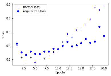
# Drawing training loss congratulations to verify loss
import matplotlib.pyplot as plt

history_dict = history.history
loss_values_normal = history_dict['val_loss']
loss_values_regularized = history_dict3['val_loss']

epochs = range(1,len(loss_values)+1)

plt.plot(epochs,loss_values_normal,'b+',label='normal loss')
plt.plot(epochs,loss_values_regularized,'bo',label='regularized loss')
plt.xlabel('Epochs')
plt.ylabel('Loss')
plt.legend()

plt.show()

#Other weight regularization can also be used

from keras import regularizers
# L1 regularization
regularizers.l1(0.001)
# Simultaneous regularization of L1 and L2
regularizers.l1_l2(l1=0.001,l2=0.001)

dropout regularization

Dropout is one of the most effective and commonly used regularization methods for neural networks. To use dropout for a certain layer is to randomly discard some output features of the layer (set to 0) in the training process. dropout rate is the proportion of features set to 0, usually 0.2-0.5.
Within the scope. This method cannot be used in testing.

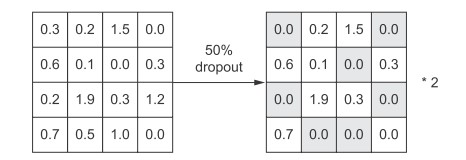
The core idea of this method is to introduce noise into the output value of the layer and break the insignificant accidental mode (Hinton calls it conspiracy). If there is no noise, the network will remember these accidental patterns. coding is implemented as follows:

##Weight regularization
from keras import models
from keras import layers
from keras import regularizers

model4 = models.Sequential()
# Each coefficient of the weight matrix increases the total network loss by 0.001 * weight_coefficient_value.
model4.add(layers.Dense(16, kernel_regularizer = regularizers.l2(0.001), activation='relu',input_shape=(10000,)))
model4.add(layers.Dropout(0.5))
model4.add(layers.Dense(16, kernel_regularizer = regularizers.l2(0.001), activation='relu'))
model4.add(layers.Dropout(0.5))
model4.add(layers.Dense(1,activation='sigmoid'))

# Standard optimizer
model4.compile(optimizer='rmsprop',
              loss = 'binary_crossentropy',
              metrics = ['accuracy']) # Monitoring accuracy in training process

history4 = model4.fit(partial_x_train,
                   partial_y_train,
                   epochs=20,
                   batch_size=512,
                   validation_data=(x_val,y_val))

history_dict4 = history4.history

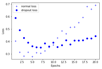
# Drawing training loss congratulations to verify loss
import matplotlib.pyplot as plt

history_dict = history.history
loss_values_normal = history_dict['val_loss']
loss_values_dropout = history_dict4['val_loss']

epochs = range(1,len(loss_values)+1)

plt.plot(epochs,loss_values_normal,'b+',label='normal loss')
plt.plot(epochs,loss_values_dropout,'bo',label='dropout loss')
plt.xlabel('Epochs')
plt.ylabel('Loss')
plt.legend()

plt.show()

Share good articles on AI, machine learning, in-depth learning and computer vision, and take notes of your own learning experience in this field. Want to go deep into the study of artificial intelligence with small partners to learn together! Get on the bus!