introduce

Machine learning is a method to solve problems that cannot be clearly coded, such as classification problems. The machine learning model will learn a pattern from the data, so we can use it to determine which class the data belongs to.

But there's a problem. How does this model work? Some people cannot accept a model with good performance because it cannot be explained. These people are concerned about interpretability because they want to ensure that the model predicts the data in a reasonable way.

Eliminating multicollinearity is a necessary step before interpreting the ML model. Multicollinearity refers to the correlation between one prediction variable and another prediction variable. Although multicollinearity does not affect the performance of the model, it will affect the interpretability of the model. If we do not remove multicollinearity, we will never know how much a variable contributes to the result. Therefore, we must eliminate multicollinearity.

This article will show you how to eliminate multicollinearity using Python.

data source

For demonstration purposes, we will use a dataset called Rain in Australia. It describes the weather characteristics of different dates and locations. This data set is also a supervised learning problem. We can use this data to predict whether it will rain tomorrow. This dataset can be found on Kaggle, where you can access it.

import pandas as pd

df = pd.read_csv('data.csv')
print(df.shape)
df.head()

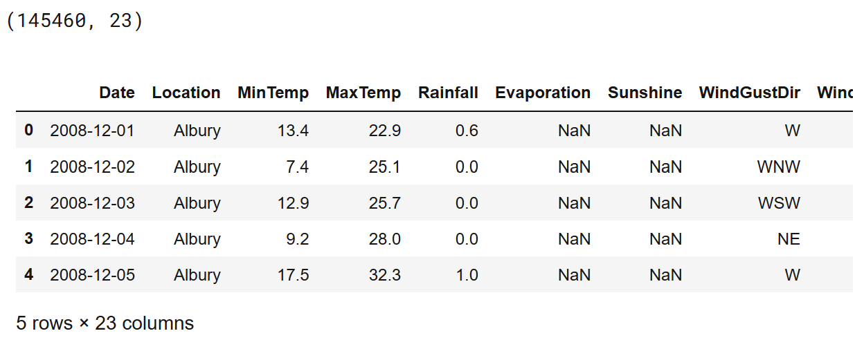
Preprocessed data

After loading the data, the next step is to preprocess the data. In this example, we will not use classification columns and delete rows that lack at least one value for each column. Here is the code to do this:

df = df[list(df.columns[2:])]
df = df.drop(['WindGustDir', 'WindDir9am', 'WindDir3pm'], axis=1)
df = df.dropna()
print(df.shape)
df.head()

Calculate VIF value

After we have clean data, let's calculate the variance expansion factor (VIF) value. What is Vif?

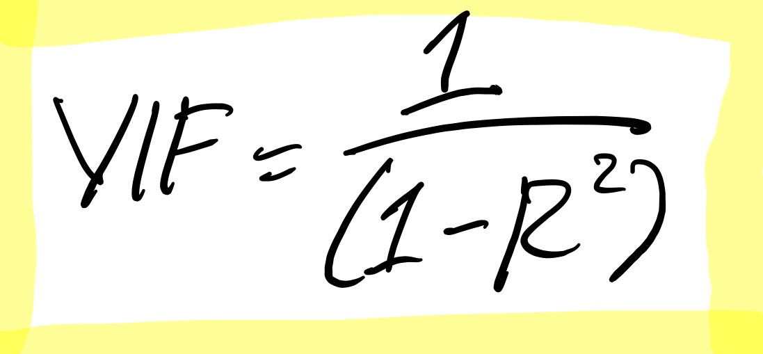
VIF is a value that determines whether a variable has multicollinearity. This figure also represents the extent to which a variable is exaggerated by its linear correlation with other variables.

The value of VIF starts from 1 and has no upper limit. If this number becomes larger, it means that this variable has huge multicollinearity.

In order to calculate the VIF, we will perform a linear regression process for each variable, where the variable will become the target variable. After we finish this process, we calculate the square of R. Finally, we use this formula to calculate the VIF value:

In Python, we can use the variance in the statmodels library_ inflation_ Factor function to calculate VIF. Here are the codes and results of doing so:

import statsmodels.api as sm
from statsmodels.stats.outliers_influence import variance_inflation_factor

X = df[list(df.columns[:-2])]

vif_info = pd.DataFrame()
vif_info['VIF'] = [variance_inflation_factor(X.values, i) for i in range(X.shape[1])]
vif_info['Column'] = X.columns
vif_info.sort_values('VIF', ascending=False)

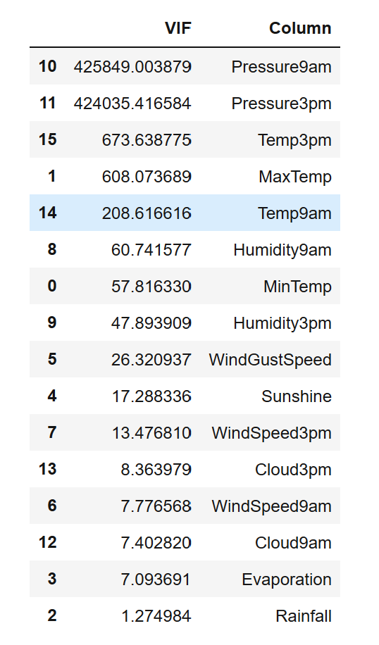
As can be seen from the above, the VIF value of almost all variables is greater than 5. Even the VIF value of pressure variable exceeds 400000. This is a big factor!

Therefore, we need to clear these multicollinearity from the data.

Eliminate Multicollinearity

To eliminate multicollinearity, we can do two things. We can create new features or delete them from the data.

Deleting features is not recommended first. Because we remove this feature, it may cause information loss. Therefore, we will first generate new features.

From the data, we can see that there are some features that have their pairs. For example, 'Temp9am' plus' Temp3pm ',' Pressure9am 'plus' Pressure3pm', 'Cloud9am' plus' Cloud3pm ', etc.

From these features, we can generate new features. The new feature will include the difference between these pairs. After we create these features, we can safely delete them from the data.

Here are the codes and results of doing so:

df['TempDiff'] = df['Temp3pm'] - df['Temp9am']
df['HumidityDiff'] = df['Humidity3pm'] - df['Humidity9am']
df['CloudDiff'] = df['Cloud3pm'] - df['Cloud9am']
df['WindSpeedDiff'] = df['WindSpeed3pm'] - df['WindSpeed9am']
df['PressureDiff'] = df['Pressure3pm'] - df['Pressure9am']

X = df.drop(['Temp3pm', 'Temp9am', 'Humidity3pm', 'Humidity9am', 'Cloud3pm', 'Cloud9am', 'WindSpeed3pm', 'WindSpeed9am', 'Pressure3pm', 'Pressure9am', 'RainToday', 'RainTomorrow'], axis=1)

X.head()

Now let's look at the VIF value of the data:

vif_info = pd.DataFrame()
vif_info['VIF'] = [variance_inflation_factor(X.values, i) for i in range(X.shape[1])]
vif_info['Column'] = X.columns
vif_info.sort_values('VIF', ascending=False)

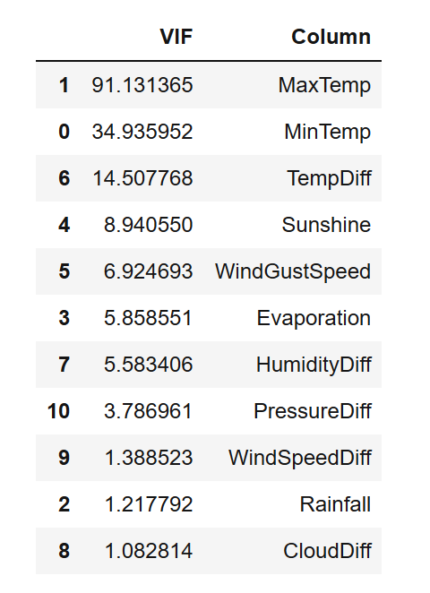
As you can see from the above, we still get variables with huge VIF values. However, we still get a good result from generating new functions.

Now let's delete features with VIF values greater than 5. Here are the codes and results of doing so:

X = X.drop(['MaxTemp', 'MinTemp', 'TempDiff', 'Sunshine'], axis=1)

vif_info = pd.DataFrame()
vif_info['VIF'] = [variance_inflation_factor(X.values, i) for i in range(X.shape[1])]
vif_info['Column'] = X.columns
vif_info.sort_values('VIF', ascending=False)

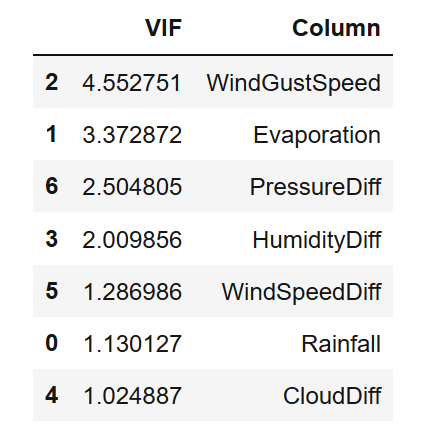
okay! Now we have all variables with VIF values less than 5. With these variables, we can now interpret the results. But first, let's build our machine learning model.

Build model

In this case, we will use support vector machine (SVM) algorithm to model our data. In short, it can create a different data plane by using SVM.

Because our data belongs to a classification task, we will use the SVC object in scikit learn to create the model. Here is the code to do this:

from sklearn.preprocessing import LabelEncoder
from sklearn.model_selection import train_test_split
from sklearn.svm import SVC

encoder = LabelEncoder()
y_encoded = encoder.fit_transform(y)
print(encoder.classes_)
print(y_encoded)

X_train, X_test, y_train, y_test = train_test_split(X.values, y_encoded)

model = SVC()
model.fit(X.values, y_encoded)

print(model.score(X_test, y_test))

Explain with the importance of arrangement characteristics

Theoretically, the support vector machine model is unexplainable. This is because we cannot interpret the results just by looking at the parameters. But fortunately, there are several ways to explain this model. One of the methods we can use is to arrange the importance of features.

The importance of a feature is measured by observing how much the error increases after changing the eigenvalue. If the change of eigenvalue increases the error of the model, the feature is important.

To implement this method, you can use permutation in the scikit learn library_ The importance function is used to calculate the importance of the feature. Based on this result, we will create a box diagram to visualize the importance of features.

Here are the codes and results of doing so:

from sklearn.inspection import permutation_importance

result = permutation_importance(model, X.values, y_encoded, n_repeats=10, random_state=42)

perm_imp_idx = result.importances_mean.argsort()
plt.boxplot(result.importances[perm_imp_idx].T, vert=False,
            labels=X.columns[perm_imp_idx])
plt.title('Feature Importance from Rain in Australia Dataset')
plt.show()

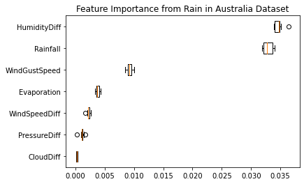
As you can see from the above, the HumanityDiff feature is the most important feature that contributes greatly to the final result. Then there is the rainfall characteristic, which is the second most important characteristic. Followed by wind gustspeed, evaporation, wind speed diff, pressure diff and cloud diff.

Final summary

do well! Now you have learned how to remove multicollinearity from a dataset using Python. I hope this article can help you eliminate multicollinearity and explain machine learning models.

By Irfan Alghani Khalid