On December 20, the central bank authorized the national interbank lending center to announce that the latest loan market quotation interest rate (LPR) is: 1-year LPR is 3.8%, down 5 BP compared with the previous period, and more than 5-year LPR is 4.65%, which is consistent with the previous period.
After "standing still" for 19 consecutive months, the 1-year LPR quotation was lowered for the first time in the year! However, the 5-year LPR quotation remains unchanged, so there is no substantive change for mortgage buyers who choose floating interest rate.
Although the five-year LPR quotation remains unchanged, which is due to the current real estate regulation tone of "housing without speculation", the houses that can not be bought still can not be bought, and the house prices in the core areas of first tier cities are still strong. How can I get the current house price in my city? Python can help you!
Taking Guangzhou, where the author is currently located, as an example, due to the tight demand for residential land supply in first tier cities, there are few new sites released every year, so the price of second-hand houses can more accurately and truly reflect the local house price market. Then we can use Python to crawl the information of second-hand houses in Guangzhou on the Internet for analysis. Here we select the data of Lianjia network for crawling.
1 Environmental preparation
Before using Python to crawl house price data for analysis, prepare the environment first.
1.1 tools
Because we need to run the code and view the results for analysis, we choose Anaconda + Jupiter notebook to write and compile the code.
Anaconda is an open-source Python distribution that contains rich scientific packages and their dependencies. It is the first choice for data analysis, so there is no need to manually import and install various dependent packages for data analysis using pip.
Jupyter Notebook is a Web application that allows users to combine descriptive text, mathematical equations, code and visual content into an easy to share document. It has become a necessary tool for data analysis and machine learning. Because it allows data analysts to focus on explaining the whole analysis process to users rather than combing documents.
The easiest way to install Jupyter Notebook is to use anaconda. Anaconda comes with Jupyter Notebook, which can be used in the default environment.
1.2 module
The modules (Libraries) mainly used in the house source data crawling and analysis include:
- requests: crawl web information
- Time: set the rest time after each climb
- Beautiful soup: parse the crawled page and get data from it
- re: regular expression operation
- pandas, numpy: process data
- matplotlib: visual analysis of data
- sklearn: cluster analysis of data
Import these related modules (Libraries):
import requests
import time
from bs4 import BeautifulSoup
import re
import pandas as pd
import numpy as np
import matplotlib.pyplot as plt
from sklearn.cluster import KMeans
Note that in the Jupiter notebook, you need to import this part of the module before you can execute the following code blocks, otherwise you will report an error that the dependent package cannot be found.
2 build crawlers to capture information
2.1 Analysis page
Before crawling data, first observe and analyze the URL structure of the web page and the structure of the data to be crawled in the target page.
2.1.1. URL structure analysis
The URL structure of the second-hand house list page of lianjia.com is:
http://gz.lianjia.com/ershoufang/pg1/
Where gz represents the city, ershoufang is the channel name and pg1 is the page code. We only climb the second-hand housing channel in Guangzhou, so the front part will not change, but the page number behind will increase monotonically from 1 to 100.
So we split the URL into two parts:
- Fixed part: http://gz.lianjia.com/ershoufang/pg
- Variable part: 1 - 100
For the variable part, we can use the for loop to generate a number of 1-100, splice it with the previous fixed part into the URL to be crawled, and then recursively integrate and save the page information crawled by each URL.
2.1.2. Page structure analysis
The data information we need to crawl includes: house location, total price, unit price, house type, area, orientation, decoration, floor, building age, building type, number of people concerned, etc. With the help of the element viewer of the browser development tool, we can see that these data information are in the info div of the page:
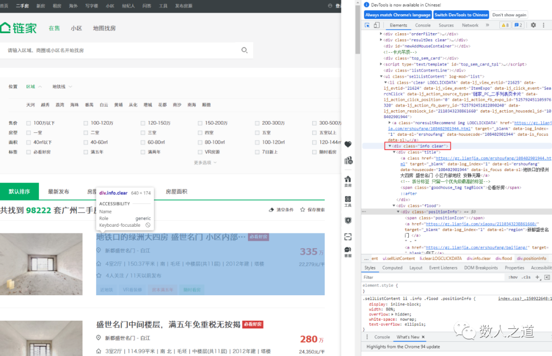
Figure 2-1-1: page structure analysis of required data
Disassemble the div where the required data is located as DOM as follows:
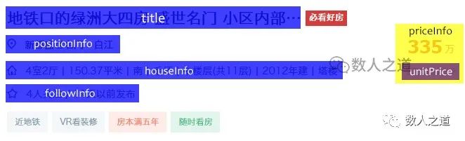
Figure 2-1-2: disassembly of div DOM where the data is located
The location information of the house is in the positionInfo tag. The house type, area, orientation, floor, building age, building type and other attribute information of the house are in the houseInfo tag. The price information of the house is in the priceInfo tag, and the attention information is in the followInfo tag.
2.2 building Crawlers
In order to disguise as a normal request as much as possible, we need to set a header in the http request, otherwise it is easy to be blocked. There are many ready-made header information on the Internet. You can also use httpwatch and other tools to view them.
# Set request header information
headers = {
'Accept':'application/json, text/javascript, */*; q=0.01',
'Accept-Encoding':'gzip, deflate, br',
'Accept-Language':'zh-CN,zh;q=0.8',
'Connection':'keep-alive',
'Referer':'http://www.baidu.com/link?url=_andhfsjjjKRgEWkj7i9cFmYYGsisrnm2A-TN3XZDQXxvGsM9k9ZZSnikW2Yds4s&wd=&eqid=c3435a7d00006bd600000003582bfd1f'
}
Use the for loop to generate a number of 1-100. After converting the format, splice it with the fixed part of the previous URL to form the URL to be crawled. Then recursively save the crawled page information, and set the request interval between each two pages to 0.5 seconds.
# Set the URL fixed section of the second-hand house list page
url = 'http://gz.lianjia.com/ershoufang/pg'

# Circular crawling of second-hand house list page information
for i in range(1, 100):
    if i == 1:
        i = str(i)
        entireURL = (url + i + '/')
        res = requests.get(url=entireURL, headers=headers)
        html = res.content
    else:
        i = str(i)
        entireURL = (url + i + '/')
        res = requests.get(url=entireURL, headers=headers)
        html2 = res.content
        html = html + html2
    # Set request interval per page
    time.sleep(0.5)
Because there are too many saved page information data, Jupyter Notebook cannot output and display all of them. You can first set the number of pages to be obtained a little less, such as 1-2 pages, and run the verification to check whether the crawling is successful:
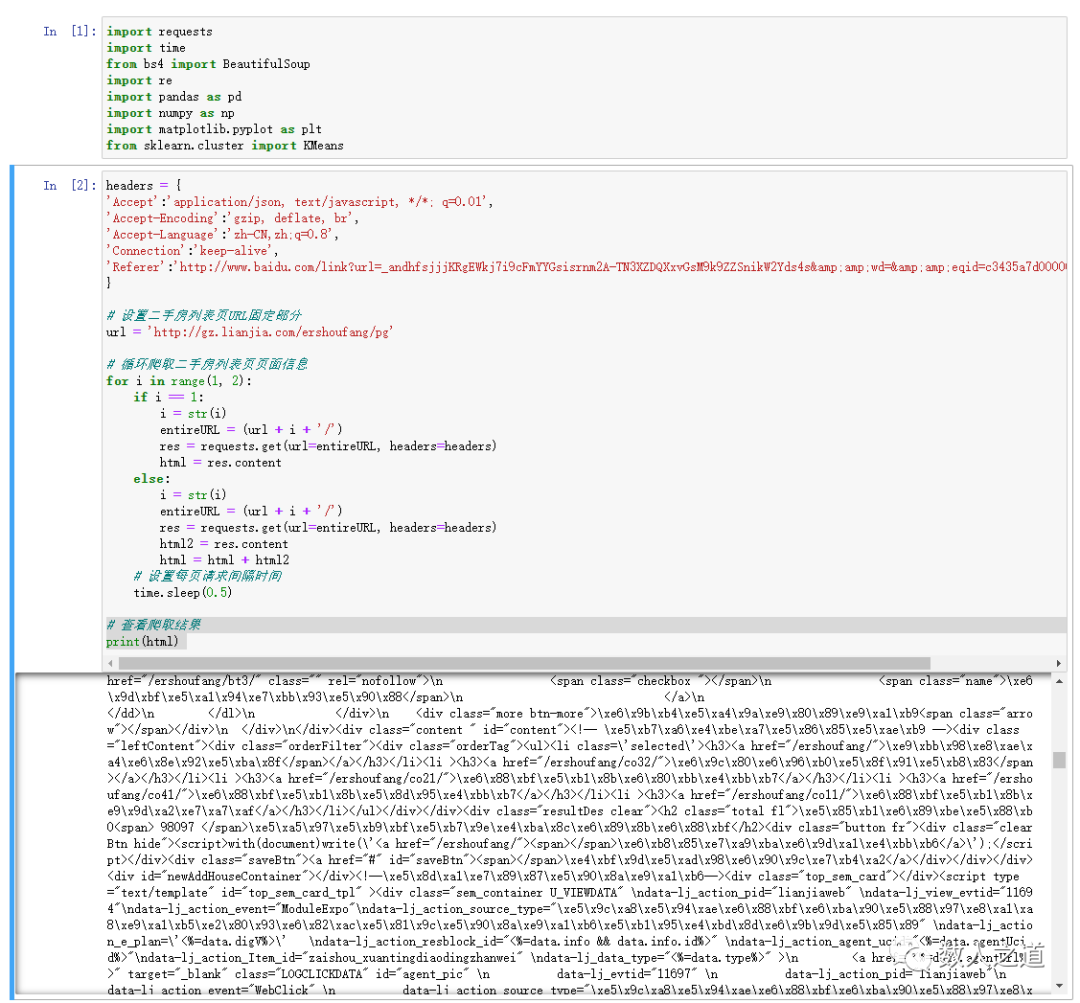
Figure 2-2-1: verifying crawling page information results
Page information has been successfully crawled.
2.3 extracting information
After page crawling is completed, it is impossible to read and extract data directly, and page parsing is also required. We use the beautiful soup module to parse the page into what we see when we view the source code in the browser (as shown on the right side of figure 2-1-1).
# Analyze the crawled page information
htmlResolve = BeautifulSoup(html, 'html.parser')
After parsing, extract the required data according to the analysis of the page structure. Next, we extract five parts of the data information of the total price (priceInfo), unit price (unitPrice), position (positionInfo), property (houseInfo) and follow info of the house supply.
Extract the part of the class=priceInfo attribute in the page div, and use the for loop to store the total price data of each house source in the array tp.
# Extract the total house price information
price = htmlResolve.find_all("div", attrs={"class": "priceInfo"})
tp = []
for p in price:
    totalPrice = p.span.string
    tp.append(totalPrice)
The method of extracting the unit price, location, attribute and attention information of houses is similar to that of extracting the total price of houses.
# Extract house unit price information
unitPriceInfo = htmlResolve.find_all("div", attrs={"class": "unitPrice"})
upi = []
for up in unitPriceInfo:
    unitPrice = up.get_text()
    upi.append(unitPrice)

# Extract house location information
positionInfo = htmlResolve.find_all("div", attrs={"class": "positionInfo"})
pi = []
for ps in positionInfo:
    position = ps.get_text()
    pi.append(position)

# Extract attribute information such as house type, area and orientation
houseInfo = htmlResolve.find_all("div", attrs={"class": "houseInfo"})
hi = []
for h in houseInfo:
    house = h.get_text()
    hi.append(house)

# Extract listing attention information
followInfo = htmlResolve.find_all("div", attrs={"class": "followInfo"})
fi = []
for f in followInfo:
    follow = f.get_text()
    fi.append(follow)
Extract several arrays and check the extracted information:
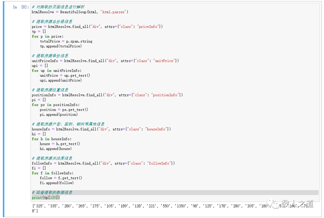
Figure 2-3-1: check data information extraction
See the first 20 data of the total price array of houses. The results are normal and the extraction is successful. The checking method of other arrays is similar.
3 processing data and structural characteristics
3.1 create data table
The pandas module is used to summarize the total price, unit price, location, attribute, attention and other information of the house supply extracted earlier, and generate a DataFrame data table for later data analysis.
# Create data table
house = pd.DataFrame({"totalprice": tp, "unitprice": upi, "positioninfo": pi, "houseinfo": hi, "followinfo": fi})
After creation, you can view the contents of the data table and check the structure of the data table:
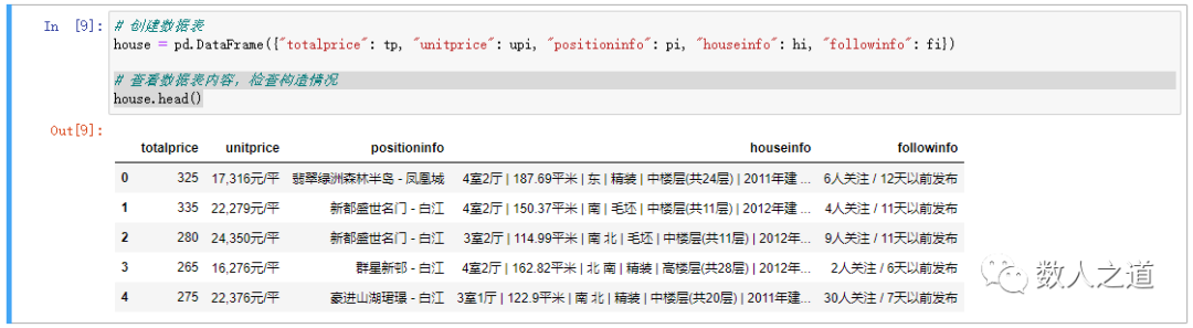
Figure 3-1-1: check the contents of the data sheet
The data table was successfully built.
3.2 structural characteristics
Although we have constructed the extracted information into the data of DataFrame structure, the data set table is relatively rough. For example, the attribute information such as house type, area and orientation of the house are contained in the house source attribute information (houseinfo) field and cannot be used directly. Therefore, we need to further process the data table.
According to the required data information, we construct new features for the fields in the data table for further analysis.
From the houseinfo field, newly constructed features: house type, area, orientation, decoration, floor, building age and building type.
From the following info field, a new feature is constructed: attention.
The method of feature construction here is to perform column operation, and cut the original large field into a new field with the minimum granularity feature.
Because the attribute information of each house source is separated by vertical lines, we only need to separate the attribute information by vertical lines.
# Feature construction of house property information
houseinfo_split = pd.DataFrame((x.split('|') for x in house.houseinfo), index=house.index, columns=["huxing","mianji","chaoxiang","zhuangxiu","louceng","louling","louxing","spec"])
Use the same method to construct the "attention" feature field of the house source. Note that the feature information separator here is a slash rather than a vertical line.
# Feature construction of house source attention information
followinfo_split = pd.DataFrame((y.split('/') for y in house.followinfo), index=house.index, columns=["guanzhu", "fabu"])
After the construction is completed, check the result table of feature field construction:
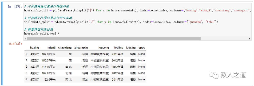
Figure 3-2-1: viewing feature field construction results
After the constructed feature fields are spliced into the original data table, these fields can be used together with other data information in the analysis.
# After splicing the constructed feature fields into the original data table
house = pd.merge(house, houseinfo_split, right_index=True, left_index=True)
house = pd.merge(house, followinfo_split, right_index=True, left_index=True)
Check the data sheet results after splicing:
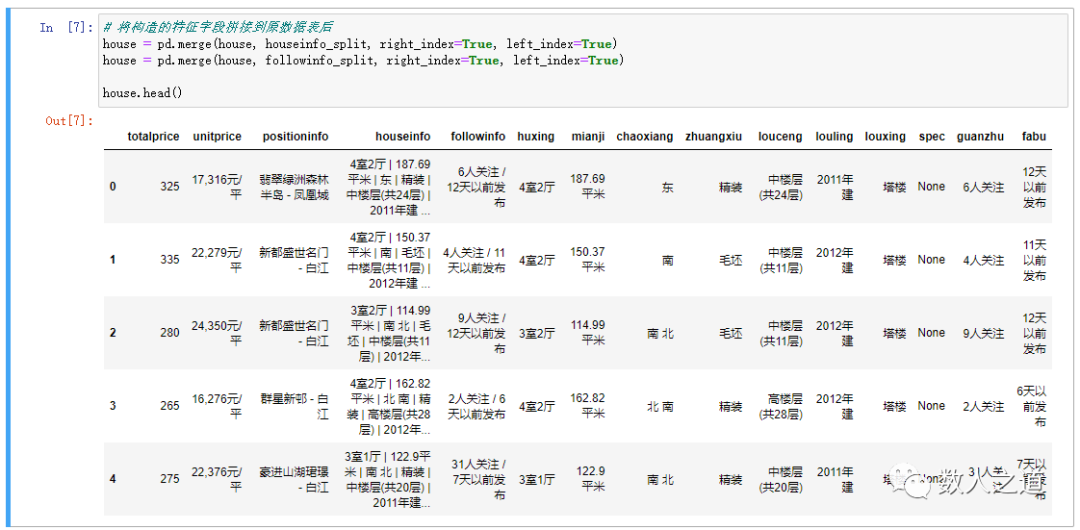
Figure 3-2-2: viewing the data sheet results after splicing
The data table after splicing contains the original information and newly constructed eigenvalues.
3.3 data processing and cleaning
In the data table after completing the splicing of eigenvalue structure, the data of some fields are mixed with numbers and Chinese, and the data format is text, which can not be used directly.
3.3.1. Data processing
The data processing work here is to extract numbers from strings. Two methods can be adopted: one is to extract the string after the number as a separator in the same way as the column; The other is to extract by regular expression.
Use the first method to extract the number of the following fields: house supply unit price.
# Feature construction of numerical housing unit price information
unitprice_num_split = pd.DataFrame((z.split('element') for z in house.unitprice), index=house.index, columns=["danjia_num","danjia_danwei"])

# After splicing the constructed feature fields into the original data table
house = pd.merge(house, unitprice_num_split, right_index=True, left_index=True)
The second method is used to extract the following fields: house area and attention.
# Define a function to extract numbers from a string
def get_num(string):
    return (re.findall("\d+\.?\d*", string)[0])

# Extract the number in the house area information
house["mianji_num"] = house["mianji"].apply(get_num)

# Extract the number in the listing attention information
house["guanzhu_num"] = house["guanzhu"].apply(get_num)
3.3.2. Data cleaning
The extracted data needs to be cleaned before use. The usual operations include removing spaces and format conversion.
Remove the spaces at both ends of the extracted house supply unit price, area and attention figures.
# Remove spaces at both ends of the extracted numeric field
house["danjia_num"] = house["danjia_num"].map(str.strip)
house["mianji_num"] = house["mianji_num"].map(str.strip)
house["guanzhu_num"] = house["guanzhu_num"].map(str.strip)
Convert all numerical fields (including the total price of houses) to float format to facilitate subsequent analysis.
# Converts the format of a numeric field to float
house["danjia_num"] = house["danjia_num"].str.replace(',', '').astype(float)
house["totalprice"] = house["totalprice"].astype(float)
house["mianji_num"] = house["mianji_num"].astype(float)
house["guanzhu_num"] = house["guanzhu_num"].astype(float)
Check the data sheet results after data processing and cleaning:
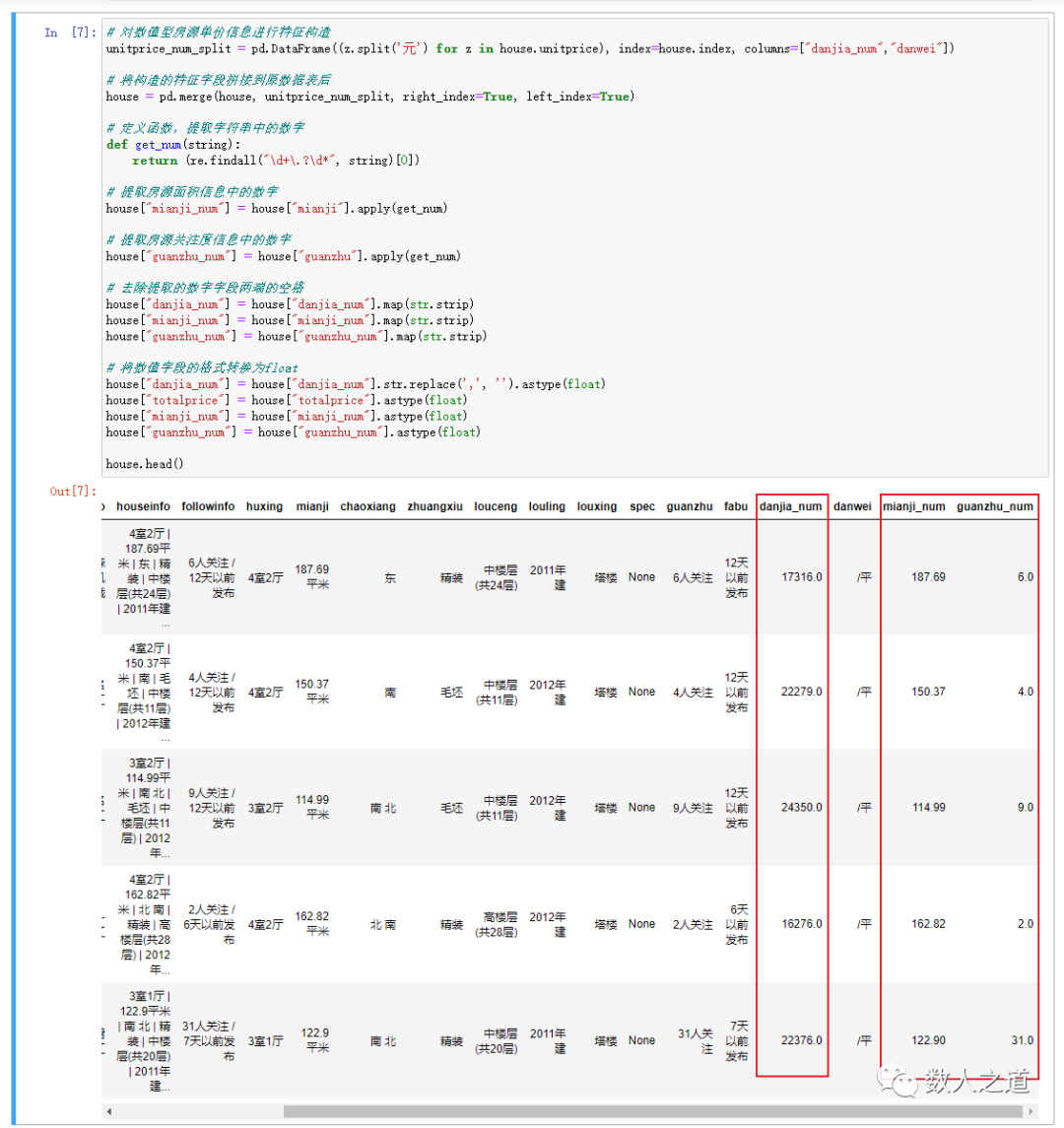
Figure 3-3-1: viewing the data sheet results after data processing and cleaning
The figures in the unit price, area and attention information of the house supply have been extracted, and the values of the total price, unit price, area and attention of the house supply have been correctly converted to float format.
4. Analyze data and visual output
After information extraction, cleaning and processing of the crawled data, the final data results can be analyzed.
Here, we explore and analyze the house price, house area and degree of attention that we are more concerned about, and use the Matplotlib module to draw 2D graphics to visually output the data.
4.1 housing area distribution
4.1.1. View range
View the housing area range of crawling data of second-hand houses on sale in Guangzhou.
# View the range of listing area data
house["mianji_num"].min(), house["mianji_num"].max()
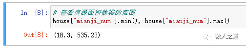
Figure 4-1-1: viewing the area range of houses
The range of housing area is obtained: (18.3, 535.23)
4.1.2. Data grouping
According to the area range of houses, the house area data are grouped. Here, taking 50 as the group distance, the house area is divided into 11 groups, and the number of houses in these 11 groups is counted.
# Group listings area data
bins = [0, 50, 100, 150, 200, 250, 300, 350, 400, 450, 500, 550]
group_mianji = ['Less than 50', '50-100', '100-150', '150-200', '200-250', '250-300', '300-350', '350-400', '400-450', '450-500', '500-550']
house['group_mianji'] = pd.cut(house['mianji_num'], bins, labels=group_mianji)

# Summarize the number of houses by house area
group_mianji = house.groupby('group_mianji')['group_mianji'].agg(len)
The effect of grouping statistics is equivalent to the following SQL statements:
select group_mianji, count(*) from house group by group_mianji;
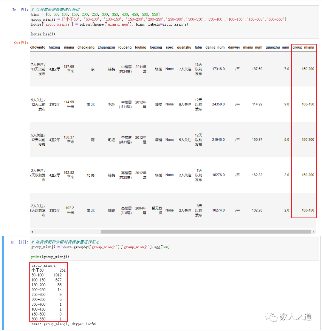
Figure 4-1-2: viewing the grouping results of housing area data
It can be seen that most houses are concentrated in the range of 50-150 square meters, which is in line with common sense.
4.1.3. Draw distribution map
Use the Matplotlib module to draw the distribution map of the number of houses grouped and counted according to the house area. In the process, the numpy module needs to be used for y-axis grouping construction.
# Draw house area distribution map
plt.rc('font', family='STXihei', size=15)
ygroup = np.array([1, 2, 3, 4, 5, 6, 7, 8, 9, 10, 11])
plt.barh([1, 2, 3, 4, 5, 6, 7, 8, 9, 10, 11], group_mianji, color='#205bc3', alpha=0.8, align='center', edgecolor='white')
plt.ylabel('Area grouping (unit: m2)')
plt.xlabel('quantity')
plt.title('Area distribution of houses')
plt.legend(['quantity'], loc='upper right')
plt.grid(color='#92a1a2', linestyle='--', linewidth=1, axis='y', alpha=0.4)
plt.yticks(ygroup, ('Less than 50', '50-100', '100-150', '150-200', '200-250', '250-300', '300-350', '350-400', '400-450', '450-500', '500-550'))

# View the plotted distribution map
plt.show()
View the drawing results of house area distribution map:
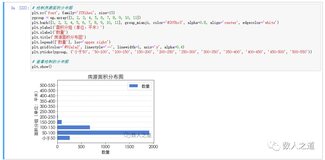
Figure 4-1-3: viewing the drawing results of house area distribution map
After the visual output of the processed data, the analysis will get twice the result with half the effort.
4.1.4. Data analysis
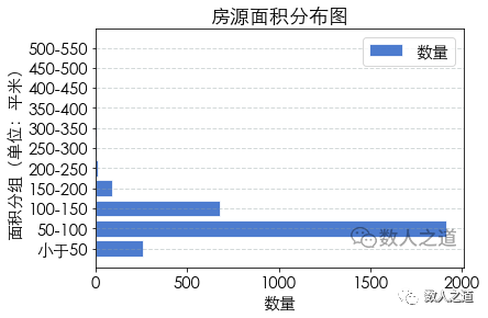
Figure 4-1-4: distribution of housing area
In the captured data of second-hand houses on sale in Guangzhou, the largest number is the houses with an area of 50-100, followed by the houses with an area of 100-150. With the increase of area, the quantity decreases; There are also a certain number of small area houses less than 50.
4.2 total price distribution of houses
4.2.1. View range
View the total price range of second-hand houses on sale in Guangzhou.
# View the range of total house price data
house["totalprice"].min(), house["totalprice"].max()
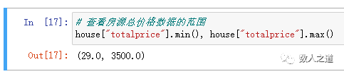
Figure 4-2-1: viewing the total price range of houses
Get the total price range of houses: (29.0, 3500.0)
4.2.2. Data grouping
Group the total price data of houses according to the total price range of houses. Here, taking 500 as the group distance, the house area is divided into 7 groups, and the number of houses in these 7 groups is counted.
# Group the total price data of houses
bins = [0, 500, 1000, 1500, 2000, 2500, 3000, 3500]
group_totalprice = ['Less than 500', '500-100', '1000-1500', '1500-2000', '2000-2500', '2500-3000', '3000-3500']
house['group_totalprice'] = pd.cut(house['totalprice'], bins, labels=group_totalprice)

# Summarize the number of houses by grouping the total price of houses
group_totalprice = house.groupby('group_totalprice')['group_totalprice'].agg(len)
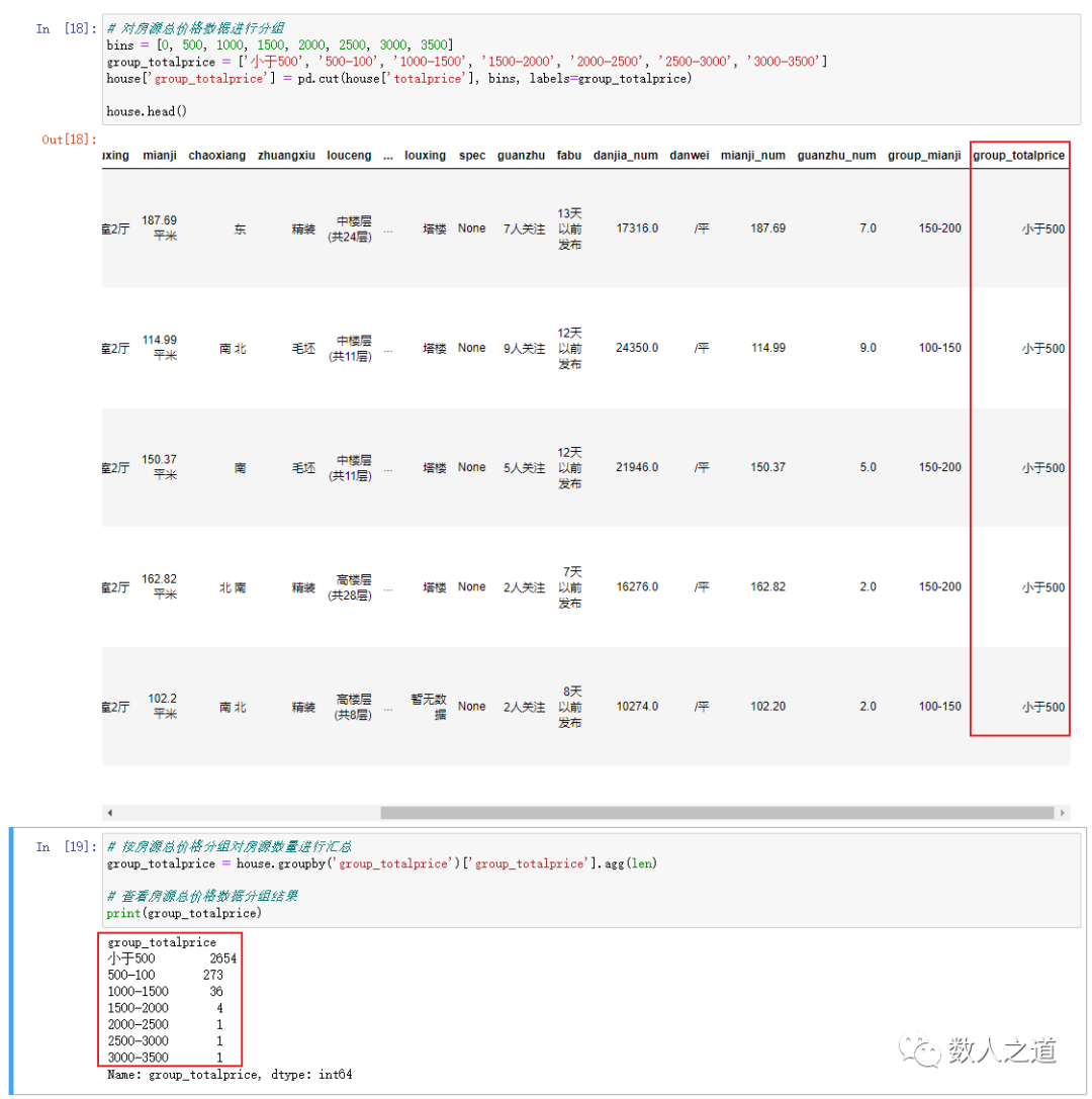
Figure 4-2-2: viewing the grouping results of total house price data
It can be seen that most of the total house prices are concentrated in the range of less than 5 million.
4.2.3. Draw distribution map
Use the Matplotlib module to draw a distribution map for the number of houses grouped and counted by the total price of houses.
# Draw the distribution map of total house price
plt.rc('font', family='STXihei', size=15)
ygroup = np.array([1, 2, 3, 4, 5, 6, 7])
plt.barh([1, 2, 3, 4, 5, 6, 7], group_totalprice, color='#205bc3', alpha=0.8, align='center', edgecolor='white')
plt.ylabel('Total price grouping (unit: 10000 yuan)')
plt.xlabel('quantity')
plt.title('Total price distribution of houses')
plt.legend(['quantity'], loc='upper right')
plt.grid(color='#92a1a2', linestyle='--', linewidth=1, axis='y', alpha=0.4)
plt.yticks(ygroup, ('Less than 500', '500-100', '1000-1500', '1500-2000', '2000-2500', '2500-3000', '3000-3500'))

# View the plotted distribution map
plt.show()
View the drawing results of the total price distribution map of houses:
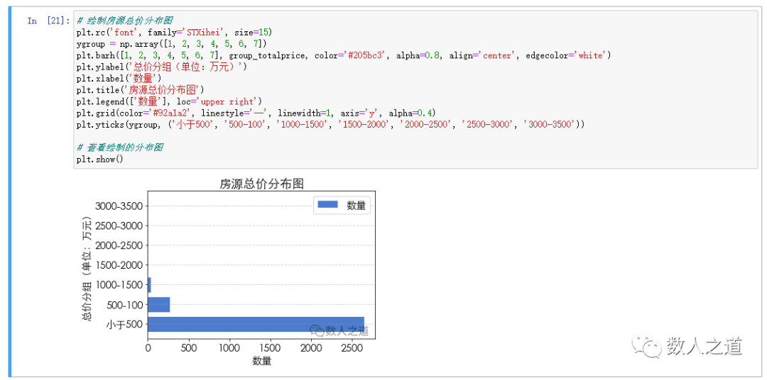
Figure 4-2-3: view the drawing results of the total price distribution map of houses
4.2.4. Data analysis
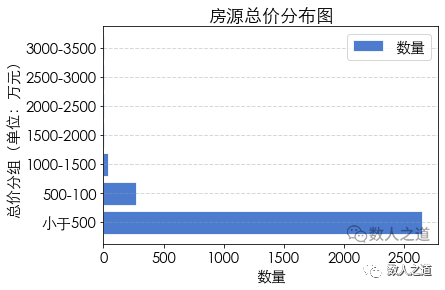
Figure 4-2-4: total price distribution of houses
In the captured data of second-hand houses on sale in Guangzhou, the largest number is the houses with a total price of less than 5 million, and far more than the houses with a total price of more than 5 million. It seems that Guangzhou is the most friendly first tier city. At least it is easier to buy a house here than the other three first tier cities.
The highest house price here is 35 million. Of course, this is not the real ceiling level of house prices in Guangzhou. This is because lianjia.com can only crawl 100 pages of data, and we can't get the records not displayed on the page. Therefore, we can't crawl all the second-hand housing data; In addition, the top luxury houses will not be listed on the public platform.
4.3 distribution of house source attention
The process of house source attention distribution analysis is similar to the distribution analysis of house source area and house source total price. Here, the process is no longer carried out, and the results of house source attention distribution map are directly viewed:
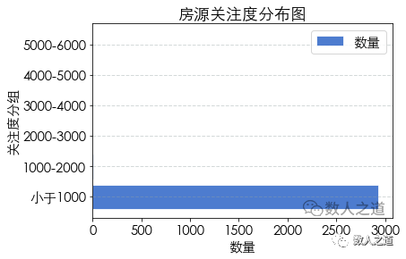
Figure 4-3-1: distribution of house supply attention
It can be seen here that the distribution map is very unbalanced due to the four houses with more than 1000 or even 5000 attention, and most of the houses have less than 1000 attention.
It should be noted that the attention data here can not accurately represent the popularity of houses. In the actual business, the hot houses are very popular, and the transaction may be concluded just after the launch. Due to the fast sale speed, there is less attention. We ignore these complex situations for the time being, so the attention data is for reference only.
4.4 cluster analysis of houses
Finally, we use the machine learning library sklearn to cluster the crawled data of second-hand houses on sale in Guangzhou according to the total price, area and attention. The second-hand houses on sale are divided into different categories according to the similarity of total price, area and attention.
# The total price, area and attention of houses are used for clustering
house_type = np.array(house[['totalprice', 'mianji_num', 'guanzhu_num']])

# Set the centroid quantity parameter value to 3
cls_house = KMeans(n_clusters=3)

# Calculate clustering results
cls_house = cls_house.fit(house_type)
View the center point coordinates of each category, and mark the category in the original data table.
# View the center coordinates of the classification results
cls_house.cluster_centers_

# Label the category of the house in the original data table
house['label'] = cls_house.labels_
View the center point coordinates of the classification results:
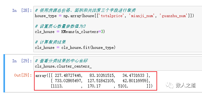
Figure 4-4-1: viewing the center coordinates of classification results
According to the central coordinates of the three categories at the three points of total price, area and attention, the second-hand houses on sale are divided into three categories:

Figure 4-4-2: classification of second-hand houses
This classification is a little contrary to our daily experience. Look at the central coordinates. The third deviation is very large. We export the data table to Excel to view this data.
# Write to Excel
house.to_excel('ershouHousePrice.xls')
After completion, you can see the generated Excel file named ershouHousePrice in the directory where the project is located. Open the file and view the data records with more than 1000 attention.

Figure 4-4-3: viewing data with attention above 1000
They are all second-hand houses from Huajing new town and Nongjiang Institute. This is suspected of brush count. Interested friends can eliminate this part of the data and analyze it to see what the difference is.
However, from the above analysis and from the perspective of marketing and regional characteristics of the market, in Guangzhou's second-hand housing market, most of the houses with total price and medium area will be better than those with low total price and area in terms of location, location, transportation, medical treatment, education and commerce. In these areas with more abundant resources, the siphon capacity of first tier cities is much stronger than that of non first tier cities. In addition, the medium level of the second-hand housing market in Guangzhou is lower than that in other first tier cities. To sum up, second-hand houses in Guangzhou with total price and medium area can attract more users' attention.
5 Conclusion
As mentioned above, because lianjia.com can only crawl 100 pages of data, we can't crawl the records not displayed on the page. Therefore, what we crawl here is not all the second-hand housing source data and can't be used as a commercial reference.
The purpose of writing this article is to attract jade, so that everyone can understand website crawlers and data analysis, and on this basis, carry out deeper and more divergent exploration, draw inferences from one instance. For example, since you can get the information of second-hand houses, you can get the information of first-hand houses. All you have to do is observe the URL and page structure of first-hand houses and modify them; Housing source analysis from different elements and angles; wait.
All codes in this article can be obtained from my github or gitee:
https://github.com/hugowong88/ershouHouseDA_gz https://gitee.com/hugowong88/ershou-house-da_gz
THE END