The loss function used in this paper is the loss function constructed by KL discretization, without formula derivation; The code part is a user-defined function, not sklearn.

The loss function constructed by discrete logistic regression KL is:  

 

Where m is the number of samples; p_1 indicates the probability that the label is 1; y^{(i)} represents the true value of the i-th sample; x^{(i)} represents the ith sample data (including multiple features, i.e. one line of data; the last value is 1).  

The derivation (gradient expression) of the loss function is:  

 

Formula derivation idea:

1. BCE can be disassembled into pairsandDerivative w and b respectively;
2. Bring the above results into,

Logistic regression custom function:

def logit_gd(X,w,y):
    """
    Returns the result of a logistic regression gradient descent
    """
    m=X.shape[0]
    return (X.T.dot(sigmoid(X.dot(w))-y))/m

How to use custom logistic regression function as prediction model? (case: label classification)

Idea:

         1. Create a custom dataset

        2. Use the logistic regression prediction label to draw the learning curve for model evaluation

1. Create a user-defined dataset. Use the user-defined function here to create a user-defined dataset  .

def arrayGenCla(num_examples=1000,num_inputs=2,num_class=3,deg_dispersion=[4,2],bias=False):
    mean_=deg_dispersion[0]  # Set data mean
    std_=deg_dispersion[1]   # Set data variance
    k=mean_*(num_class-1)/2   # Set the penalty factor to adjust the data to be distributed around the origin
    cluster_l=np.empty([num_examples,1])
    lf=[]
    ll=[]
    
    for i in range(num_class):   # Create data for each category
        data_temp=np.random.normal(i*mean_-k,std_,size=(num_examples,num_inputs))
        lf.append(data_temp)
        labels_temp=np.full_like(cluster_l,i)
        ll.append(labels_temp)
    
    features=np.concatenate(lf) # Merge classified data
    labels=np.concatenate(ll)
    
    if bias== True: # If the set dataset is multivariate, add "1" to the last column of features
        features=np.concatenate((features,np.ones(labels.shape)),1)
    
    return features,labels

  2. Use the logistic regression prediction label to draw the learning curve for model evaluation

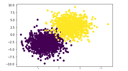
First, create a dataset using a custom function. The dataset has two labels with less overlap.  

np.random.seed(9)
f,l=arrayGenCla(num_class=2,deg_dispersion=[6,2],bias=True)
plt.scatter(f[:,0],f[:,1],c=l)
plt.show()

Then, the data set is segmented into training set and test set. The gradient descent is used to solve the parameter W, save the results after each w iteration, calculate the model performance in the training set and test set, and draw the learning curve.

Part of the code is a user-defined function, which is added behind the learning curve.

X_train,X_test,y_train,y_test=array_split(f,l,random_state=9)

X_train[:,:-1]=z_score(X_train[:,:-1])
X_test[:,:-1]=z_score(X_test[:,:-1])

np.random.seed(24)
w=np.random.randn(f.shape[1],1)

score_train=[]
score_test=[]
for i in range(num_epoch):
    w=sgd_cal(X_train,w,y_train
              ,logit_gd
              ,batch_size=batch_size
              ,epoch=1
              ,lr=lr_init*lr_lambda(i))
    score_train.append(logit_acc(X_train,w,y_train,thr=0.5))
    score_test.append((logit_acc(X_test,w,y_test,thr=0.5)))

plt.plot(range(num_epoch),score_train,label='score_train')
plt.plot(range(num_epoch),score_test,label='score_test')
plt.legend()
plt.show()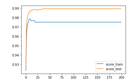

def logit_cla(yhat, thr=0.5):
    """
    Return logistic regression category output function
    """
    ycla = np.zeros_like(yhat)
    ycla[yhat >= thr] = 1
    return ycla

def logit_acc(X,w,y,thr=0.5):
		"""
		Return the evaluation index of logistic regression
		"""
    y_hat=sigmoid(X.dot(w))
    y_cal=logit_cla(y_hat,thr=thr)
    return(y_cal==y).mean()

Conclusion: according to the learning curve, after about 25 iterations, the parameter W has been close to the optimal solution, and the model tends to be stable. The factors considered in the model setting are relatively simple, w which performs better in the test set, which is accidental.

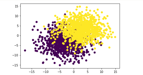
If the data overlap more, how will this logistic regression model perform? Next, experiment again:

# Performance results of logistic regression on data sets with large degree of coincidence

np.random.seed(9)
f_1,l_1=arrayGenCla(num_class=2,deg_dispersion=[6,4],bias=True)
plt.scatter(f_1[:,0],f_1[:,1],c=l)
plt.show()

X_train,X_test,y_train,y_test=array_split(f_1,l_1,random_state=9)

X_train[:,:-1]=z_score(X_train[:,:-1])
X_test[:,:-1]=z_score(X_test[:,:-1])

np.random.seed(24)
w=np.random.randn(f.shape[1],1)

score_train=[]
score_test=[]
for i in range(num_epoch):
    w=sgd_cal(X_train,w,y_train
              ,logit_gd
              ,batch_size=batch_size
              ,epoch=1
              ,lr=lr_init*lr_lambda(i)
             )
    score_train.append(logit_acc(X_train,w,y_train,thr=0.5))
    score_test.append((logit_acc(X_test,w,y_test,thr=0.5)))

plt.plot(range(num_epoch),score_train,label='score_train')
plt.plot(range(num_epoch),score_test,label='score_test')
plt.legend()
plt.show()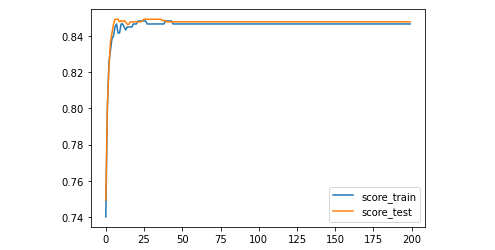

Conclusion: according to the learning curve, after 25 iterations, the model tends to be stable, and the accuracy decreases to about 0.85.