Given the error function, learning rate, and even the size of the target variable, the training neural network may become unstable. Large updating of weights during training will lead to numerical overflow or underflow, which is usually called gradients exploding.
Gradient explosion is more common in recurrent neural networks, such as LSTM, because the accumulation of gradient expands over hundreds of input time steps.
A common and relatively easy solution to gradient explosion is to change the derivative of the error before propagating the error backward through the network and using it to update the weight. The two methods include: giving the selected vector norm to rescale the gradient; And clipping gradient values beyond the preset range. Together, these methods are called gradient clipping.
1. Gradient explosion and cutting
The neural network is trained by random gradient descent optimization algorithm. This requires first estimating the loss on one or more training samples, and then calculating the derivative of the loss, which is back propagated through the network to update the weight. A small part of the back propagation error controlled by the learning rate is used to update the weight.
The update of the weight may be so large that the numerical accuracy of the weight exceeds or falls below this numerical accuracy. The weight can take "NaN" or "Inf" value in case of overflow or underflow, but the network will be useless because the NaN value is always predicted when the signal flows through the invalid weight. Weight overflow or underflow refers to the instability of the network training process, and the unstable training process makes the network unable to train, resulting in the model is essentially useless, so it is called gradient explosion.
In a given neural network (such as convolutional neural network or multilayer perceptron), gradient explosion may occur due to improper configuration selection:
Improper selection of learning rate will lead to large weight update.
The prepared data has a lot of noise, resulting in great differences in target variables.
Improper selection of loss function leads to large error value.
Gradient explosion is easy to occur in recurrent neural networks (such as long-term and short-term memory networks). In general, explosion gradients can be avoided by carefully configuring the network model, for example, selecting a smaller learning rate and scaling the target variable and standard loss function proportionally. Nevertheless, for recursive networks with a large number of input time steps, gradient explosion is still a problem that needs to be considered.
A common solution to gradient explosion is to change the error derivative first, then back propagate the error derivative through the network, and then use it to update the weight. By rescaling the error derivative, the weight update will also be rescaled, which greatly reduces the possibility of overflow or underflow. There are two main methods to update the error derivative:
Gradient Scaling
Gradient Clipping
Gradient scaling involves normalizing the error gradient vector so that the vector norm size is equal to a defined value, such as 1.0. As long as they exceed the threshold, rescale them. If the gradient exceeds the expected range, gradient clipping forces the gradient value (element by element) to a specific minimum or maximum. These methods are usually referred to as gradient clipping.
When the traditional gradient descent algorithm proposes a very large step size, gradient clipping reduces the step size to small enough that it is unlikely to go beyond the region of the steepest descent direction of the gradient.
It is a method that only solves the numerical stability of the training depth neural network model, but can not improve the network performance.
The value of gradient vector norm or preset range can be configured through repeated experiments. The common values used in the literature can be used, or the general vector norm or range can be observed through experiments, and then a reasonable value can be selected.
The same gradient clipping configuration is usually used for all layers in the network. However, in some examples, a wider range of error gradients is allowed in the output layer than in the hidden layer.
2. TensorFlow.Keras implementation
2.1 Gradient Norm Scaling
Gradient norm scaling: when the L2 vector norm (sum of squares) of the gradient vector exceeds the threshold, change the derivative of the loss function to have a given vector norm.
For example, you can specify a norm of 1.0, which means that if the vector norm of the gradient exceeds 1.0, the values in the vector are rescaled so that the vector norm equals 1.0. In Keras, this is achieved by specifying the clipnorm parameter on the optimizer:
....
opt = SGD(lr=0.01, momentum=0.9, clipnorm=1.0)
2.2 Gradient Value Clipping
If the gradient value is less than the negative threshold or greater than the positive threshold, the gradient value cuts the derivative of the loss function to a given value. For example, you can specify a norm of 0.5, which means that if the gradient value is less than - 0.5, it is set to - 0.5, and if the gradient value is greater than 0.5, it is set to 0.5. By specifying the clipvalue parameter on the optimizer:
...
opt = SGD(lr=0.01, momentum=0.9, clipvalue=0.5)
3. Examples
A simple MLP regression problem is used to illustrate the role of gradient clipping.
3.1 gradient explosion MLP
from sklearn.datasets import make_regression
from keras.layers import Dense
from keras.models import Sequential
from keras.optimizers import SGD
import matplotlib.pyplot as plt
plt.rcParams['figure.dpi'] = 150
# Construct regression problem data set
X, y = make_regression(n_samples=1000, n_features=20, noise=0.1, random_state=1)
# Divide training set and verification set
n_train = 500
trainX, testX = X[:n_train, :], X[n_train:, :]
trainy, testy = y[:n_train], y[n_train:]
# Define model
model = Sequential()
model.add(Dense(25, input_dim=20, activation='relu', kernel_initializer='he_uniform'))
model.add(Dense(1, activation='linear'))
# Compiling model
model.compile(loss='mean_squared_error', optimizer=SGD(lr=0.01, momentum=0.9))
# Training model
history = model.fit(trainX, trainy, validation_data=(testX, testy), epochs=100, verbose=0)
# Evaluation model
train_mse = model.evaluate(trainX, trainy, verbose=0)
test_mse = model.evaluate(testX, testy, verbose=0)
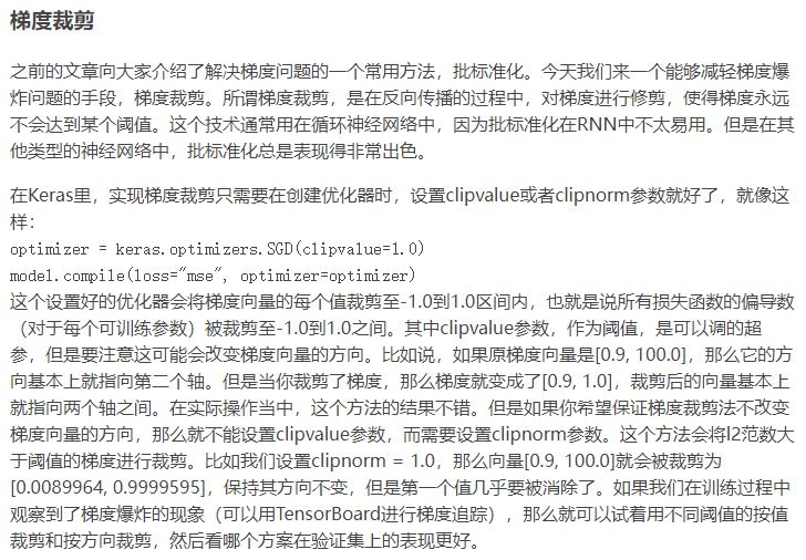
print('Train: %.3f, Test: %.3f' % (train_mse, test_mse))
# Draw loss curve
plt.title('Mean Squared Error')
plt.plot(history.history['loss'], label='train')
plt.plot(history.history['val_loss'], label='test')
plt.legend()
plt.show()
In this case, the model cannot be learned, resulting in the prediction of NaN value. Given a very large error, and then update the calculated error gradient for the weight in the training, the model weight will explode. The traditional solution is to use standardization or normalization to readjust the target variables. However, this article uses an alternative method, gradient pruning.
3.2 gradient norm scaling MLP
from sklearn.datasets import make_regression
from keras.layers import Dense
from keras.models import Sequential
from keras.optimizers import SGD
import matplotlib.pyplot as plt
plt.rcParams['figure.dpi'] = 150
# Construct regression problem data set
X, y = make_regression(n_samples=1000, n_features=20, noise=0.1, random_state=1)
# Divide training set and verification set
n_train = 500
trainX, testX = X[:n_train, :], X[n_train:, :]
trainy, testy = y[:n_train], y[n_train:]
# Define model
model = Sequential()
model.add(Dense(25, input_dim=20, activation='relu', kernel_initializer='he_uniform'))
model.add(Dense(1, activation='linear'))
# Compiling model
opt = SGD(lr=0.01, momentum=0.9, clipnorm=1.0)
model.compile(loss='mean_squared_error', optimizer=opt)
# Training model
history = model.fit(trainX, trainy, validation_data=(testX, testy), epochs=100, verbose=0)
# Evaluation model
train_mse = model.evaluate(trainX, trainy, verbose=0)
test_mse = model.evaluate(testX, testy, verbose=0)
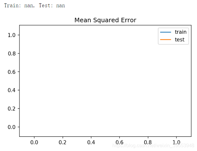
print('Train: %.3f, Test: %.3f' % (train_mse, test_mse))
# Draw loss curve
plt.title('Mean Squared Error')
plt.plot(history.history['loss'], label='train')
plt.plot(history.history['val_loss'], label='test')
plt.legend()
plt.show()
The figure shows that the loss decreases rapidly from a large value of more than 20000 to a small value of less than 100 within 20 epoch s.
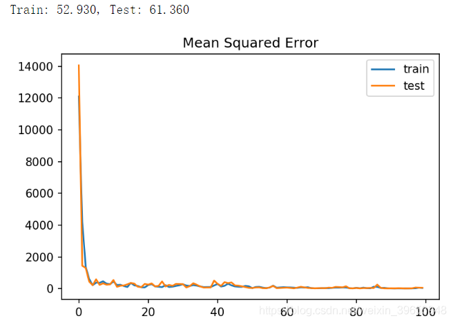
3.3 gradient value clipping MLP
from sklearn.datasets import make_regression
from keras.layers import Dense
from keras.models import Sequential
from keras.optimizers import SGD
import matplotlib.pyplot as plt
plt.rcParams['figure.dpi'] = 150

# Construct regression problem data set
X, y = make_regression(n_samples=1000, n_features=20, noise=0.1, random_state=1)

# Divide training set and verification set
n_train = 500
trainX, testX = X[:n_train, :], X[n_train:, :]
trainy, testy = y[:n_train], y[n_train:]

# Define model
model = Sequential()
model.add(Dense(25, input_dim=20, activation='relu', kernel_initializer='he_uniform'))
model.add(Dense(1, activation='linear'))

# Compiling model
opt = SGD(lr=0.01, momentum=0.9, clipvalue=5.0)
model.compile(loss='mean_squared_error', optimizer=opt)

# Training model
history = model.fit(trainX, trainy, validation_data=(testX, testy), epochs=100, verbose=0)

# Evaluation model
train_mse = model.evaluate(trainX, trainy, verbose=0)
test_mse = model.evaluate(testX, testy, verbose=0)
print('Train: %.3f, Test: %.3f' % (train_mse, test_mse))

# Draw loss curve
plt.title('Mean Squared Error')
plt.plot(history.history['loss'], label='train')
plt.plot(history.history['val_loss'], label='test')
plt.legend()
plt.show()