AlexNet Preface Knowledge

The Macro Framework of Deep Learning: training and inference and Their Application Scenarios
json.loads() method of loading json data: used to convert str-type data to dict.

• Training

For example, now you want to train a model that can distinguish between an apple and an orange. You need to search for some pictures of the apple and an orange. These pictures together are called training dataset. The training dataset has labels. The labels of the apple pictures are apples and the same is true of oranges. An initial neural network makes itself more accurate by constantly optimizing its own parameters. It may start with 10 pictures of apples, only 5 of which are considered apples by the network, and 5 of which are mistaken. At this time, by optimizing the parameters, the other 5 errors will become right. This whole process is called training.

• Inference

You've trained a model and it works well in the training dataset, but we expect it to recognize pictures it hasn't seen before. If you take a new picture and throw it into the network for judgment, it is called live data. If the accuracy of the field data is very high, then your network training is very good. We take the trained model out for a walk and call it Inference.

• deployment

To apply a trained neural network model, you need to put it on a hardware platform and make sure it runs. This process is called deployment.

(1) alexnet_inference.py analysis

1.1 transforms.Compose()

# hard code
    # The mean and std of three RGB channels are obtained by ImageNet data statistics.
    norm_mean = [0.485, 0.456, 0.406]  # Through the ImageNet statistics, it is RGB three channels(mean and std).
    norm_std = [0.229, 0.224, 0.225]
    # Transforms. Compose (): Image preprocessing package in Pytorch that combines multiple steps
    inference_transform = transforms.Compose([
        transforms.Resize(256),
        transforms.CenterCrop((224, 224)),
        transforms.ToTensor(),
        transforms.Normalize(norm_mean, norm_std),
    ])

transforms.Compose()
The following describes the functions in transforms:

• Resize: Resize a given picture to given size
• Normalize: Normalized an tensor image with mean and standard deviation
• ToTensor: Converts a PIL image or an array of shapes [H, W, C] whose range of values is [0,225] into a tensor of shapes [C, H, W], whose range of values is [0, 1.0] (torch.FloadTensor)
• ToPILImage: convert a tensor to PIL image
• Scale: Not used anymore, Resize is recommended
• CenterCrop: Clip in the middle of the image
• RandomCrop: Clipping at a random location
• RandomHorizontalFlip: Flips a given PIL image at a 0.5 probability level
• RandomVerticalFlip: Flips a given PIL image vertically with a probability of 0.5
• RandomResizedCrop: Clips the PIL image to any size and aspect ratio, and then transforms it to a given size
• Grayscale: Convert an image to a grayscale image
• RandomGrayscale: Converts an image to a grayscale with a certain probability
• FiceCrop: Cut the image into four corners and one center
• TenCrop
• Pad: Fill all edges of the image with the given pad value
• ColorJitter: Randomly change the brightness contrast and saturation of the image.

1.2 unsqueeze_()

    # path --> img
    # Loading pictures 
    #If not used. convert('RGB') converts to read an image with RGBA four channels and A channel transparent
    img_rgb = Image.open(path_img).convert('RGB') 

    # img --> tensor
    img_tensor = img_transform(img_rgb, inference_transform)
    img_tensor.unsqueeze_(0)        # [c,h,w] increase to [b,c,h,w]
    # to(device): the tensor variable copy at the beginning of reading the data is copied to the GPU specified by device, and subsequent operations are performed on the GPU.
    img_tensor = img_tensor.to(device)

    return img_tensor, img_rgb

PIL Image Processing Standard Library - convert('RGB')
unsqueeze_in pytorch Usage of (increasing dimension)
Pytorch Learn Notes - to(device) usage

1.3 AlexNet(nn.Module)

nn.AdaptiveAvgPool2d()
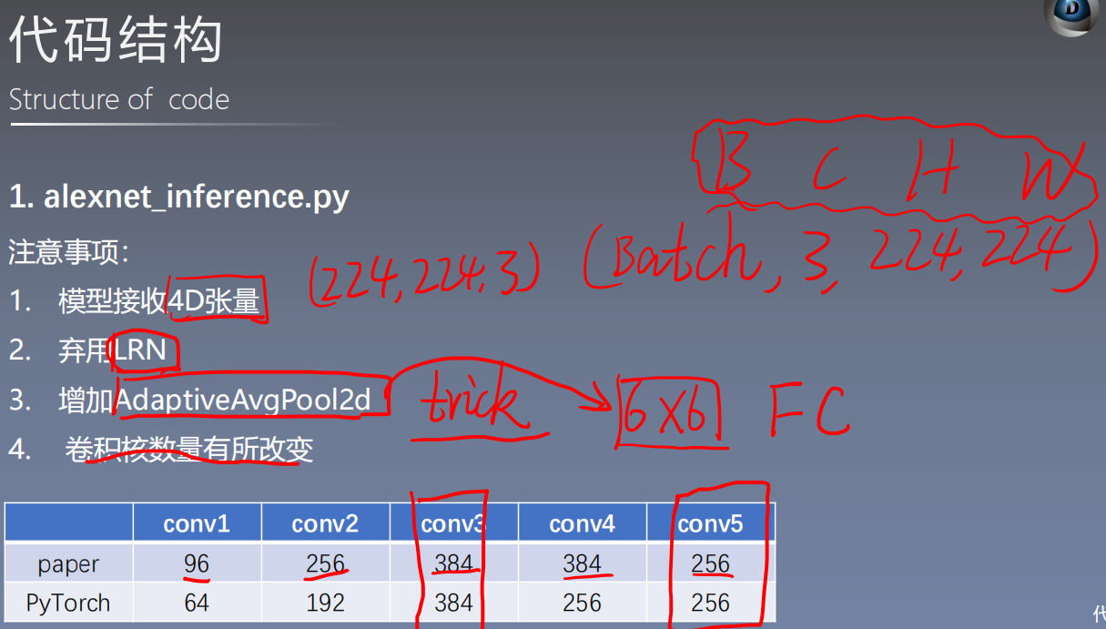
AlexNet in Pytorch changes the number of convolution cores in the original paper

class AlexNet(nn.Module):

    def __init__(self, num_classes: int = 1000) -> None:
        super(AlexNet, self).__init__()
        self.features = nn.Sequential(
            # conv1 
            nn.Conv2d(3, 64, kernel_size=11, stride=4, padding=2),  # 96 --> 64
            nn.ReLU(inplace=True),
            nn.MaxPool2d(kernel_size=3, stride=2), # 3 > 2 
            
			# conv2
            nn.Conv2d(64, 192, kernel_size=5, padding=2),# 384 --> 256
            nn.ReLU(inplace=True),
            nn.MaxPool2d(kernel_size=3, stride=2),
            
			# conv3
            nn.Conv2d(192, 384, kernel_size=3, padding=1),
            nn.ReLU(inplace=True),
            
            # conv4
            nn.Conv2d(384, 256, kernel_size=3, padding=1),
            nn.ReLU(inplace=True),
            
            # conv5
            nn.Conv2d(256, 256, kernel_size=3, padding=1),
            nn.ReLU(inplace=True),
            nn.MaxPool2d(kernel_size=3, stride=2),
        )
        # Adaptive Average Pooling, Specified Output (H, W)
        self.avgpool = nn.AdaptiveAvgPool2d((6, 6)) # trick 
        self.classifier = nn.Sequential(
            nn.Dropout(),
            nn.Linear(256 * 6 * 6, 4096),
            nn.ReLU(inplace=True),
            
            nn.Dropout(),
            nn.Linear(4096, 4096),
            nn.ReLU(inplace=True),
            
            nn.Linear(4096, num_classes),
        )

    def forward(self, x: torch.Tensor) -> torch.Tensor:
        x = self.features(x)
        x = self.avgpool(x)
        x = torch.flatten(x, 1)
        x = self.classifier(x)
        return x

1.4 Loading pretrained_model parameter for pre-training State_ Dict

Model in Pytorch. The role of Eval
Using summary in torchsummary on Pytorch

def get_model(path_state_dict, vis_model=False):
    """
    Create a model, load parameters
    :param path_state_dict:
    :return:
    """
    model = models.alexnet()
    pretrained_state_dict = torch.load(path_state_dict)
    model.load_state_dict(pretrained_state_dict)  # Parameters of Import Pre-training Model
    model.eval() # Because we are not training, we use this to keep the model parameters unchanged.

    if vis_model:
        from torchsummary import summary
        # Summy Print Shows Network Structure and Parameters
        summary(model, input_size=(3, 224, 224), device="cpu")

    model.to(device)
    return model

1.5 inference

torch.no_grad and validation mode

    # 3/5 inference  tensor --> vector
    torch.no_grad():# By adding this to forward propagation, you can speed up operations and reduce memory consumption, since forward propagation does not require calculating gradients
    with torch.no_grad():
        time_tic = time.time()
        outputs = alexnet_model(img_tensor) # Pass pictures directly to the model
        time_toc = time.time()

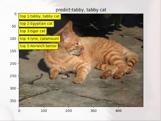
1.6 Output Top 1 and Top5 probabilities

# 4/5 index to class names
    _, pred_int = torch.max(outputs.data, 1) # Pred_ Index corresponding to int:Top-1
    _, top5_idx = torch.topk(outputs.data, 5, dim=1) # Top5_ Index corresponding to idx:Top-5

    pred_idx = int(pred_int.cpu().numpy()) 
    pred_str, pred_cn = cls_n[pred_idx], cls_n_cn[pred_idx] # Find pred_ Name of the label corresponding to the idx:Top-5 index
    print("img: {} is: {}\n{}".format(os.path.basename(path_img), pred_str, pred_cn))
    print("time consuming:{:.2f}s".format(time_toc - time_tic))

1.7 Image Display

# 5/5 visualization
    plt.imshow(img_rgb)
    plt.title("predict:{}".format(pred_str))
    top5_num = top5_idx.cpu().numpy().squeeze()
    text_str = [cls_n[t] for t in top5_num]
    for idx in range(len(top5_num)):
        plt.text(5, 15+idx*30, "top {}:{}".format(idx+1, text_str[idx]), bbox=dict(fc='yellow'))
    plt.show()

Output As Following: