Follow the up Master of station b to learn and sort out: 2.1 official demo of pytorch (lenet)_ Beep beep beep_ bilibili

catalogue

1, The rudiment of CNN -- LeNet network structure

2, Official website demo file

3, Code implementation

1.model.py

2.train.py

3.predict.py

1, The rudiment of CNN -- LeNet network structure

In 1998, LeCun et al. Released the LeNet network, thus unveiling the veil of deep learning. The subsequent deep neural networks are improved on this basis, and their structure is shown in the figure.

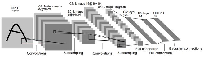
  As shown in the figure, LeNet is sequentially connected by volume layer, pool layer and full connection layer. Each layer in the network uses a differentiable function to transfer the activation data from one layer to another.

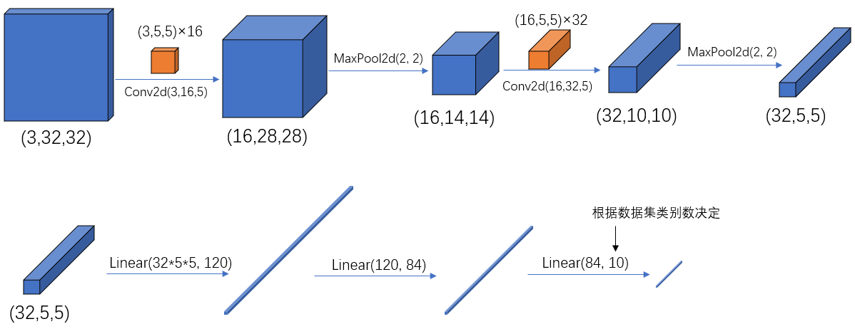
• In pytorch, the channels of tensor (i.e. input / output layer) are sorted as: [batch, channel, height, width]
• The meanings and positions of convolution, pooling and parameters in the input / output layer in pytorch are shown in the following figure:

2, Official website demo file

The LeNet demo file given on the official website of pytorch is shown in the figure:

• model.py -- define the LeNet network model
• train.py -- load the data set and train, calculate the loss value loss in the training set, calculate the accuracy in the test set, and save the trained network parameters
• predict.py -- after using the trained network parameters, use the images you find for classification test

3, Code implementation

1.model.py

# Use torch.nn package to build neural network
import torch.nn as nn
import torch.nn.functional as F

class LeNet(nn.Module): 					# It inherits from the parent class nn.Module
    def __init__(self):						# Initialize network structure
        super(LeNet, self).__init__()    	# Multi inheritance requires the super function
        self.conv1 = nn.Conv2d(3, 16, 5)
        self.pool1 = nn.MaxPool2d(2, 2)
        self.conv2 = nn.Conv2d(16, 32, 5)
        self.pool2 = nn.MaxPool2d(2, 2)
        self.fc1 = nn.Linear(32*5*5, 120)
        self.fc2 = nn.Linear(120, 84)
        self.fc3 = nn.Linear(84, 10)

    def forward(self, x):			 # Forward propagation process
        x = F.relu(self.conv1(x))    # input(3, 32, 32) output(16, 28, 28)
        x = self.pool1(x)            # output(16, 14, 14)
        x = F.relu(self.conv2(x))    # output(32, 10, 10)
        x = self.pool2(x)            # output(32, 5, 5)
        x = x.view(-1, 32*5*5)       # output(32*5*5)
        x = F.relu(self.fc1(x))      # output(120)
        x = F.relu(self.fc2(x))      # output(84)
        x = self.fc3(x)              # output(10)
        return x

The convolution layer function Conv2d in the code corresponds to the original function in pytorch:

torch.nn.Conv2d(in_channels,
                out_channels, 
                kernel_size, 
                stride=1,
                padding=0, 
                dilation=1, 
                groups=1, 
                bias=True, 
                padding_mode='zeros')

The input parameters are explained as follows:  

• in_channels: enter the depth of the characteristic matrix. If you input an RGB color image, it is in_channels=3
• out_channels: the depth of the output characteristic matrix after convolution is equal to the number of convolution kernels. The depth of the output characteristic matrix using N convolution kernels is n-dimensional
• kernel_size: the size of convolution kernel. For example, if the convolution kernel is 3x3, the kernel_size=3
• Stripe: the step size of the convolution kernel. The default is 1
• padding: fill zero around the input characteristic matrix. The default value is 0
• bias: whether to use offset. The default value is true

The calculation formula of dimension change of output matrix after convolution is as follows:

• The input picture size is WxW (generally speaking, width=height)
• Filter size FxF
• Step S
• The pixel value of padding is P

If N calculated by the above formula is not an integer in the convolution process, pytorch will generally delete redundant rows and columns to ensure that the matrix size N of convolution output is an integer. For details, refer to Detailed explanation of convolution operation in pytorch

Flattening of Tensor: view()

After passing through the second pooling layer, the data is still a three-dimensional tensor(32,5,5). It needs to be flattened into (35 * 5 * 5) and then transferred to the full connection layer. The flattening operation is realized through the view() function.

2.train.py

Import package

import torch
import torchvision
import torch.nn as nn
from model import LeNet
import torch.optim as optim
import torchvision.transforms as transforms

Data preprocessing

Use the transform function to preprocess the input image data, and ToTensor() converts it into a tensor. Normalize() normalizes it

transform = transforms.Compose(
        [transforms.ToTensor(), #
         transforms.Normalize((0.5, 0.5, 0.5), (0.5, 0.5, 0.5))])

Data set introduction

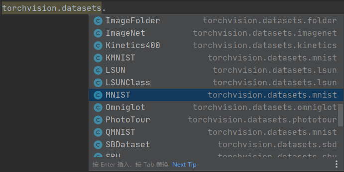
Using the torchvision.datasets function, you can download the datasets imported into pytorch online, including some common datasets, such as MNIST.

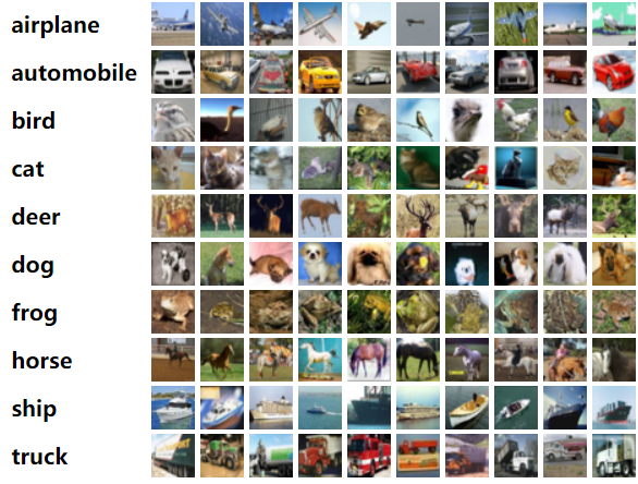
  CIFAR10 data set is used in this demo, which is a classic image classification data set. A small data set for identifying universal objects organized by Hinton's students Alex Krizhevsky and IIya Sutskever, which contains 10 categories of RGB color pictures.

  To import and load training sets:

# 50000 training pictures
    # The first time you use it, you need to set download to True to automatically download the dataset
    train_set = torchvision.datasets.CIFAR10(root='./data', train=True,
                                             download=True, transform=transform)
    train_loader = torch.utils.data.DataLoader(train_set, batch_size=36,
                                               shuffle=True, num_workers=0)

Import and load test sets:

 # 10000 verification pictures
    # The first time you use it, you need to set download to True to automatically download the dataset
    val_set = torchvision.datasets.CIFAR10(root='./data', train=False,
                                           download=False, transform=transform)
    val_loader = torch.utils.data.DataLoader(val_set, batch_size=10000,
                                             shuffle=False, num_workers=0)

  Training process parameters:

noun	definition
epoch	One epoch indicates that all samples in the training set have passed one pass
iteration	Represents one iteration, and the parameters of the network structure are updated once each iteration
batch_size	The training set is divided into multiple batches of training, and the size of each batch of data is batch_size, that is, the sample size used in one iteration

Taking this demo as an example, the training set has a total of 50000 samples, batch_size=50, so the complete training sample is once: iteration=1000  . The training process code is as follows:

net = LeNet()						  				# Define the network model of training
loss_function = nn.CrossEntropyLoss() 				# The loss function is defined as cross entropy loss function 
optimizer = optim.Adam(net.parameters(), lr=0.001)  # Define optimizer (training parameters, learning rate)

for epoch in range(5):  # One epoch is to train the whole training set once
    running_loss = 0.0
    time_start = time.perf_counter()
    
    for step, data in enumerate(train_loader, start=0):   # Traverse the training set, and step starts from 0
        inputs, labels = data 	# Get the images and labels of the training set
        optimizer.zero_grad()   # Clear history gradient
        
        # forward + backward + optimize
        outputs = net(inputs)  				  # Forward propagation
        loss = loss_function(outputs, labels) # Calculate loss
        loss.backward() 					  # Back propagation
        optimizer.step() 					  # Optimizer update parameters

        # Print time-consuming, loss, accuracy and other data
        running_loss += loss.item()
        if step % 1000 == 999:    # Print every 1000 Mini batches, once every 1000 steps
            with torch.no_grad(): # In the following steps (in the verification process), the loss gradient of each node is not calculated to prevent memory occupation
                outputs = net(test_image) 				 # The test set is transferred to the network (test_batch_size=10000), and the output dimension is [10000,10]
                predict_y = torch.max(outputs, dim=1)[1] # The index (label) corresponding to the maximum position of the median value in the output is used as the prediction output
                accuracy = (predict_y == test_label).sum().item() / test_label.size(0)
                
                print('[%d, %5d] train_loss: %.3f  test_accuracy: %.3f' %  # Print epoch, step, loss, accuracy
                      (epoch + 1, step + 1, running_loss / 500, accuracy))
                
                print('%f s' % (time.perf_counter() - time_start))        # Printing time
                running_loss = 0.0

print('Finished Training')

# Save the training parameters
save_path = './Lenet.pth'
torch.save(net.state_dict(), save_path)

The training time is about 12 minutes, and the training results are as follows:

3.predict.py

import torch
import torchvision.transforms as transforms
from PIL import Image
from model import LeNet


def main():
    transform = transforms.Compose(
        [transforms.Resize((32, 32)),
         transforms.ToTensor(),
         transforms.Normalize((0.5, 0.5, 0.5), (0.5, 0.5, 0.5))])

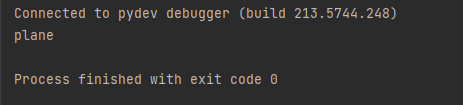
    classes = ('plane', 'car', 'bird', 'cat',
               'deer', 'dog', 'frog', 'horse', 'ship', 'truck')

    net = LeNet() # initialization
    net.load_state_dict(torch.load('Lenet.pth'))  #Load the trained weight file

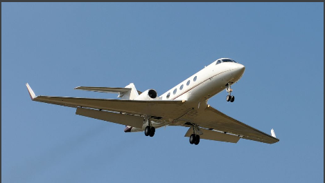
    im = Image.open('1.jpg')
    im = transform(im)  # [C, H, W]
    im = torch.unsqueeze(im, dim=0)  # [N, C, H, W]

    with torch.no_grad():
        outputs = net(im)
    #     predict = torch.max(outputs, dim=1)[1].data.numpy()
    # print(classes[int(predict)])
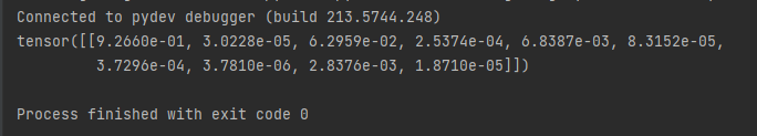
        predict = torch.softmax(outputs, dim=1)
    print(predict)


if __name__ == '__main__':
    main()

Test picture:

Test results:

  Using softmax function processing, the probability distribution of predicting the category of the figure can be obtained as follows. The index corresponding to the maximum probability value in the output result is the index of the prediction label. It can also be seen that the probability of classifying the aircraft is about 92.7%:

  Summary: CPU training is really slow!

Reference blog: pytorch image classification: 2.pytorch official demo implements a classifier (LeNet)_fun1024-CSDN blog