Fourier transform, also known as Fourier transform, means that a function satisfying certain conditions can be expressed as a trigonometric function (sine and / or cosine function) or a linear combination of their integrals. This paper will introduce how to realize the Fourier transform of image through OpenCV. You can refer to what you need

Two dimensional discrete Fourier transform (DFT)

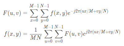
For two-dimensional image processing, x, y, x, YX and y are usually used to represent discrete spatial domain coordinate variables, and u, V, u, VU and V are used to represent discrete frequency domain variables. Two dimensional discrete Fourier transform (DFT) and inverse transform (IDFT) are:

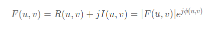
The two-dimensional discrete Fourier transform can also be expressed in polar coordinates:

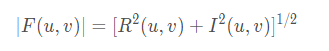
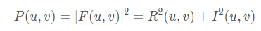
The Fourier spectrum is:

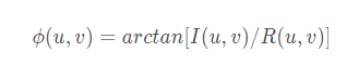
The Fourier phase spectrum is:

The Fourier power spectrum is:

Spatial sampling and frequency interval correspond to each other. The interval between discrete variables corresponding to frequency domain is: Δ u=1/M Δ T, Δυ= 1/N Δ Z. That is, the interval between samples in the frequency domain is inversely proportional to the product of the interval between spatial samples and the number of samples.

Spatial domain filters and frequency domain filters also correspond to each other. The two-dimensional convolution theorem is the link to establish an equivalent relationship between spatial domain and frequency domain filters:

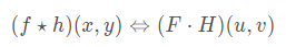
This shows that f and H are Fourier transforms of F and h, respectively; The Fourier transform of the spatial convolution of F and H is the product of their transforms.

OpenCV realizes image Fourier transform (cv.dft)

Use cv. In OpenCV DFT () function can also realize the Fourier transform of image, CV IDFT () function realizes the inverse Fourier transform of image.

Function Description:

cv.dft(src[, dst[, flags[, nonzeroRows]]]) → dst
cv.idft(src[, dst[, flags[, nonzeroRows]]]) → dst

　　

Parameter Description:

src: input image, single channel gray image, using NP Float32 format

dst: output image. The image size is the same as src, and the data type is determined by flag

flag: conversion identifier

cv. DFT_ Invert: replace the default forward transform with one-dimensional or two-dimensional inverse transform

cv.DFT_SCALE: scale indicator, which calculates the scaling result according to the number of elements. It is often associated with DFT_ Use with invert

cv.DFT_ROWS: forward or reverse Fourier transform is performed on each row of the input matrix. It is often used for complex operations such as three-dimensional or high-dimensional transformation

cv.DFT_COMPLEX_OUTPUT: forward transform the one-dimensional or two-dimensional real array. The default method is the complex array represented by two channels. The first channel is the real part and the second channel is the imaginary part

cv.DFT_REAL_OUTPUT: inverse transformation of one-dimensional or two-dimensional complex array, and the result is usually a complex matrix with the same size

matters needing attention:

1. The input image src is NP Float32 format, such as image, using NP Uint8 format must be converted to NP Float32 format.

2. Default method cv DFT_ COMPLEX_ When output, the input src is NP The output dst is a two-dimensional array of two channels. The first channel dft[:,:,0] is the real part, and the second channel dft[:,:,1] is the imaginary part.

3. It cannot be directly used to display images. You can use cv The magnitude() function converts the result of Fourier transform to gray scale [0255].

4.idft(src, dst, flags) is equivalent to DFT (SRC, DST, flags = dft_invert).

5.OpenCV realizes Fourier transform, and the calculation speed is faster than Numpy.

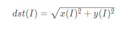
Convert the identifier to CV DFT_ COMPLEX_ When output, CV The output of the DFT () function is a two-dimensional array of two channels, using cv The magnitude () function can calculate the amplitude of two-dimensional vector.

Function Description:

cv.magnitude(x, y[, magnitude]) → dst

　　

Parameter Description:

x: A one-dimensional or multi-dimensional array that also represents the real part of a complex number, floating point

y: A one-dimensional or multi-dimensional array, which also represents the imaginary part of a complex number. It is a floating-point type. The size of the array must be the same as x

dst: output array. The array size and data type are the same as x. the operation formula is:

The value range of Fourier transform and related operations may not be suitable for image display, and normalization processing is required. CV. In OpenCV Normalize() function can realize image normalization.

Function Description:

cv.normalize(src, dst[, alpha[, beta[, norm_type[, dtype[, mask]]]]]) → dst

　　

Parameter Description:

src: input image

dst: output result, the same size and type as the input image

alpha: the minimum value after normalization; optional; the default value is 0

beta: the maximum value after normalization; optional; the default value is 1

norm_type: normalization type

• NORM_INF: Linf norm (maximum of absolute value)
• NORM_L1: L1 norm (sum of absolute values)
• NORM_L2: L2 norm (Euclidean distance), default type
• NORM_MINMAX: linear scaling, common type

dtype: optional. The default value is - 1, indicating that the output matrix is the same as the input image type

Mask: mask, optional, no mask by default

Fourier transform theoretically requires O(MN) ² Second operation, very time-consuming; The fast Fourier transform only needs O(MN ㏒ (MN)) operations.

Fourier transform function CV in OpenCV DFT () has the best computational performance for a matrix whose number of rows and columns can be decomposed into 2^p*3^q*5^r. In order to improve the operation performance, 0 can be added to the right and bottom of the original matrix to meet the decomposition condition. CV. In OpenCV Getoptimaldftsize() function can realize the optimal DFT size expansion of the image, which is applicable to CV DFT () and NP fft. fft2().

Function Description:

cv.getOptimalDFTSize(versize) → retval

　　

Parameter Description:

Versione: array size

retval: optimal array size for DFT expansion

Sample code

# 8.11: OpenCV realizes the discrete Fourier transform of two-dimensional image
imgGray = cv2.imread("../images/Fig0424a.tif", flags=0)  # flags=0 is read as a grayscale image
 
# cv2. Fourier transform of image based on DFT
imgFloat32 = np.float32(imgGray)  # Convert image to float32
dft = cv2.dft(imgFloat32, flags=cv2.DFT_COMPLEX_OUTPUT)  # Fourier transform
dftShift = np.fft.fftshift(dft)  # Move the low frequency component to the center of the frequency domain image
 
# Amplitude spectrum
# ampSpe = np.sqrt(np.power(dft[:,:,0], 2) + np.power(dftShift[:,:,1], 2))
dftAmp = cv2.magnitude(dft[:,:,0], dft[:,:,1])  # Amplitude spectrum, uncentralized
dftShiftAmp = cv2.magnitude(dftShift[:,:,0], dftShift[:,:,1])  # Amplitude spectrum, centralization
dftAmpLog = np.log(1 + dftShiftAmp)  # Logarithmic transformation of amplitude spectrum for easy display
# Phase spectrum
phase = np.arctan2(dftShift[:,:,1], dftShift[:,:,0])  # Calculated phase angle (radian system)
dftPhi = phase / np.pi*180  # Convert phase angle to [- 180, 180]
 
print("dftMag max={}, min={}".format(dftAmp.max(), dftAmp.min()))
print("dftPhi max={}, min={}".format(dftPhi.max(), dftPhi.min()))
print("dftAmpLog max={}, min={}".format(dftAmpLog.max(), dftAmpLog.min()))
 
# cv2.idft implementation of image inverse Fourier transform
invShift = np.fft.ifftshift(dftShift)  # Switch the low frequency reversal back to the four corners of the image
imgIdft = cv2.idft(invShift)  # Inverse Fourier transform
imgRebuild = cv2.magnitude(imgIdft[:,:,0], imgIdft[:,:,1])  # Reconstructed image
 
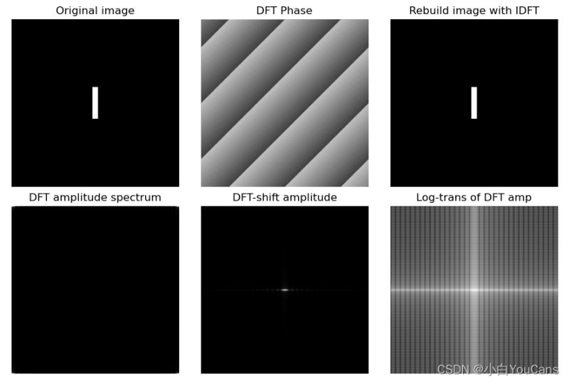
plt.figure(figsize=(9, 6))
plt.subplot(231), plt.title("Original image"), plt.axis('off')
plt.imshow(imgGray, cmap='gray')
plt.subplot(232), plt.title("DFT Phase"), plt.axis('off')
plt.imshow(dftPhi, cmap='gray')
plt.subplot(233), plt.title("Rebuild image with IDFT"), plt.axis('off')
plt.imshow(imgRebuild, cmap='gray')
plt.subplot(234), plt.title("DFT amplitude spectrum"), plt.axis('off')
plt.imshow(dftAmp, cmap='gray')
plt.subplot(235), plt.title("DFT-shift amplitude"), plt.axis('off')
plt.imshow(dftShiftAmp, cmap='gray')
plt.subplot(236), plt.title("Log-trans of DFT amp"), plt.axis('off')
plt.imshow(dftAmpLog, cmap='gray')
plt.tight_layout()
plt.show()

　　

The above is the whole content of this article. I hope it can help you.