Background introduction
All stochastic optimization algorithms (GA, ABC, PSO, STA, simulated annealing) are a routine
- Generating a pile of new candidate solutions through the current solution or some is called generating candidate solutions
- Then update the solution through an evaluation function (evaluation standard), that is, find the good one or some in a pile
- Keep cycling until the termination conditions are met
operator
The so-called operator is actually a rule for generating candidate solutions. You can understand that if you give an operator a certain input, he will return one or more candidate solutions to you
Operator description of continuous STA
There are four basic operators, namely, rotation transformation, expansion transformation, axial transformation and translation transformation
Rotation transformation
A new solution is generated by using the rotation transformation formula. Physically, it is a solution to the hypersphere with Best as the center and alpha as the radius
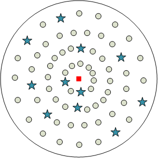
Telescopic transformation
The scaling transformation formula generates a new solution. Physically, it is possible to scale every dimension of Best to (- ∞, + ∞), and then constrain it to the boundary of the definition domain, which belongs to global search
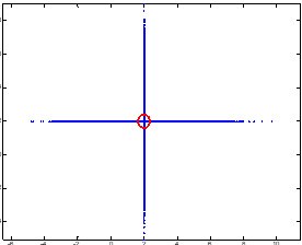
Axial transformation
The new solution is generated by using the axial transformation formula. Physically, it is possible to scale a single dimension of Best to (- ∞, + ∞), which belongs to local search and enhances the single-dimensional search ability
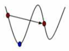
Translation transformation
The new solution is generated by using the translation formula. Physically, the new solution is generated by searching on the line oldBest newBest. We believe that there is a high probability that a good solution will appear on the connection between the old and new optimal solutions. For example, when the two solutions are on both sides of the valley bottom, the above figure is scaled in only one dimension
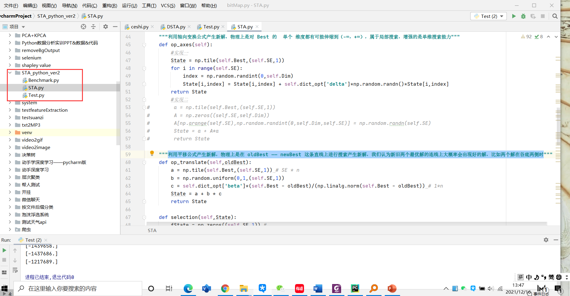
file structure
code
benchmark.py
#!/usr/bin/env python3
# -*- coding: utf-8 -*-

from functools import reduce
from operator import mul
import numpy as np
import math


def Sphere(s):
	square = map(lambda y: y * y ,s)
	return sum(square)

def Rosenbrock(s):
	square = map(lambda x, y: 100 * (y - x**2)**2 + (x - 1)**2 , s[:len(s)-1],s[1:len(s)])
	return  sum(square)

def Rastrigin(s):
	square = map(lambda x: x**2 - 10 * math.cos(2*math.pi*x) + 10, s)
	return  float(sum(square))

def Michalewicz(s):
	n = len(s)
	t1 = -sum(map(lambda x, y: math.sin(x) * (math.sin( y*x**2/math.pi ))**20, s, range(1,n+1)))
	return t1

def Griewank(s):
	t1 = sum(map(lambda x: 1/4000 * x**2, s))
	n = len(s)
	t2 = map(lambda x, y: math.cos(x/np.sqrt(y)), s, range(1,n+1))
	t3 = reduce(mul, t2)
	return t1 - t3 + 1
STA.py
# -*- coding: utf-8 -*-
"""
Created on Sat Nov  6 10:57:13 2021

@author: Intelligent control and optimization decision-making research group, School of automation, Central South University
"""

import numpy as np
import time

class STA():
    # initialization
    def __init__(self,funfcn,Range,SE,Maxiter,dict_opt):
        self.funfcn = funfcn
        self.Range = Range
        self.SE = SE
        self.Maxiter = Maxiter
        self.dict_opt = dict_opt
        self.Dim = self.Range.shape[1]

    def initialization(self):
        self.Best = np.array(self.Range[0,:] + self.Range[1,:]-self.Range[1,:]*np.random.uniform(0,1,(1,self.Range.shape[1])))
        self.fBest = self.funfcn(self.Best[0])
        self.history = []
        self.history.append(self.fBest)

    """Using the rotation transformation formula to produce a new solution is physically correct Best Center alpha Sample the hypersphere of radius SE A solution"""
    def op_rotate(self):
        R1 = np.random.uniform(-1,1,(self.SE,self.Dim))
        R2 = np.random.uniform(-1,1,(self.SE,1))
        a = np.tile(self.Best,(self.SE,1))
        b = np.tile(R2,(1,self.Dim))
        c = R1/np.tile(np.linalg.norm(R1,axis=1,keepdims = True),(1,self.Dim))
        State = a + self.dict_opt['alpha']*b*c
        return State

    """Using the expansion transformation formula to produce a new solution is physically correct Best Every dimension of can be scaled to(-∞,+∞),Then it is constrained to the boundary of the definition domain, which belongs to global search"""
    def op_expand(self):
        a = np.tile(self.Best,(self.SE,1))
        b = np.random.randn(self.SE,self.Dim)
        State = a + self.dict_opt['gamma'] * b * a
        return State

    """Using the axial transformation formula to produce a new solution is physically correct Best A single dimension of can scale to(-∞,+∞),It belongs to local search and enhances the ability of one-dimensional search"""
    def op_axes(self):
        #Realize one
        State = np.tile(self.Best,(self.SE,1))
        for i in range(self.SE):
            index = np.random.randint(0,self.Dim)
            State[i,index] = State[i,index] + self.dict_opt['delta']*np.random.randn()*State[i,index]
        return State
        #Implementation II
#        a = np.tile(self.Best,(self.SE,1))
#        A = np.zeros((self.SE,self.Dim))
#        A[np.arange(self.SE),np.random.randint(0,self.Dim,self.SE)] = np.random.randn(self.SE)
#        State = a + A*a
#        return State

    """Using the translation formula to generate a new solution is physically oldBest - newBest Search on this line to generate a new solution. We believe that there is a high probability that a good solution will appear on the connection between the old and new optimal solutions, such as when the two solutions are on both sides of the valley bottom"""
    def op_translate(self,oldBest):
        a = np.tile(self.Best,(self.SE,1)) # SE * n
        b = np.random.uniform(0,1,(self.SE,1))
        c = self.dict_opt['beta']*(self.Best - oldBest)/(np.linalg.norm(self.Best - oldBest)) # 1*n
        State = a + b * c
        return State

    def selection(self,State):
        fState = np.zeros((self.SE,1)) #
        for i in range(self.SE):
            fState[i] = self.funfcn(State[i,:])
        index = np.argmin(fState)
        return State[index,:],fState[index,:]

    def bound(self,State):
        Pop_Lb = np.tile(self.Range[0],(State.shape[0],1))
        Pop_Ub = np.tile(self.Range[1],(State.shape[0],1))
        changeRows = State > Pop_Ub
        State[changeRows] = Pop_Ub[changeRows]
        changeRows = State < Pop_Lb
        State[changeRows] = Pop_Lb[changeRows]
        return State

    def run(self):
        time_start = time.time()
        self.initialization()
        for i in range(self.Maxiter):
            if self.dict_opt['alpha'] < 1e-4:
                self.dict_opt['alpha'] = 1.0
            else:
                self.dict_opt['alpha'] = 0.5*self.dict_opt['alpha']

            """The three operators are used to generate a new solution and update the optimal solution"""
            dict_op = {"rotate": self.op_rotate(), "expand": self.op_expand(),"axes": self.op_axes()}
            for key in dict_op:
                oldBest = self.Best
                State = self.bound(dict_op[key])
                newBest, fnewBest = self.selection(State)
                if fnewBest < self.fBest:      # If the operator (any one of the three) produces a better solution than history, call the translate operator again to see if it can find a better solution
                    self.fBest, self.Best = fnewBest, newBest
                    State = self.bound(self.op_translate(oldBest))
                    newBest, fnewBest = self.selection(State)
                    if fnewBest < self.fBest:
                        self.fBest, self.Best = fnewBest, newBest

            self.history.append(self.fBest[0])
            print("The first{}The optimal value of this iteration is:{:.5e}".format(i,self.fBest[0]))

            # "" "let the algorithm stop in advance if the update amount of the two optimal values is less than 1e-10" ""
            # if (abs(self.history[i+1] - self.history[i]) < 1e-10) & (self.dict_opt['alpha'] < 1e-4):
            #     self.history = np.array(self.history[1:])
            #     break
        time_end = time.time()
        print("The total time is:{:.5f}".format(time_end - time_start))
Test.py
# -*- coding: utf-8 -*-
"""
Created on Sat Nov  6 10:57:13 2021

@author: Intelligent control and optimization decision-making research group, School of automation, Central South University
"""

from STA import STA
import Benchmark
import numpy as np
import matplotlib.pyplot as plt

#Parameter setting
funfcn = Benchmark.Sphere
Dim = 100
Range = np.repeat([-30,30],Dim).reshape(-1,Dim)
SE = 30
Maxiter = 1000
dict_opt = {'alpha':1,'beta':1,'gamma':1,'delta':1}
# Algorithm call
sta = STA(funfcn,Range,SE,Maxiter,dict_opt)
sta.run()
# Drawing
#x = np.arange(1,Maxiter+2).reshape(-1,1)
y = sta.history
x = np.arange(len(y)).reshape(-1,1)
plt.semilogy(x,y,'b-o')
plt.xlabel('Ierations')
plt.ylabel('fitness')
plt.show()
result
This is the of the Sphere function

Postscript
You can change the function test by yourself. You can see more test functions Unconstrained benchmark function , test by writing functions