1, Algorithm Introduction

   Decision Tree is a decision analysis method to obtain the probability that the expected value of net present value is greater than or equal to zero, evaluate the project risk and judge its feasibility by forming a Decision Tree on the basis of knowing the occurrence probability of various situations. It is a graphical method of intuitive application of probability analysis. Because this decision-making branch is drawn as a graph, which is very similar to the branches of a tree, it is called Decision Tree.
  in machine learning, decision tree is a prediction classification model, which is widely used in various prediction classification scenarios. It is a very common classification method. Decision tree is a kind of supervised learning, which can calculate information gain through different algorithms, and create decision tree based on it.

2, Data set information

  in this blog, we use the Titanic data set to train and evaluate the decision tree model.
  the data set mainly contains the following information:

Attribute name	describe
PassengerId	Passenger id
Survived	Survive
Pclass	Ticket grade
Name	Passenger name
Sex	Passenger gender
Age	Passenger age
SibSp	Number of non lineal relatives
Parch	Number of lineal relatives
Ticket	Ticket number
Fare	Ticket price
Cabin	cabin
Embarked	Landing port

  there are 891 records.

3, Algorithm flow and code implementation

1. Loading data sets and selection of eigenvalues

   load the dataset by implementing the function loadDataSet().

func loadDataSet(trainScale int) ([][]string, [][]string, []string) {

	file, err := os.Open("titanic.csv")
	if err != nil {
		fmt.Println("Error:", err)
		return nil, nil, nil
	}

	defer func(file *os.File) {
		err := file.Close()
		if err != nil {

		}
	}(file)

	reader := csv.NewReader(file)

	var features []string
	var trainDataSet [][]string
	var testDataSet [][]string

	temp, _ := reader.Read()
	
    /** Read feature**/

	curr := 0

	for {
		record, err := reader.Read()

		if err == io.EOF {
			break
		} else if err != nil {
			fmt.Println("Error:", err)
			return nil, nil, nil
		}

		var tempRecord []string

		/** Read the training set and test set, and cut and clean the data**/

		curr++
	}

	return trainDataSet, testDataSet, features
}

  then we cut and clean the data set. In the analysis of eigenvalues, we can find that passenger id (PassengerId), passenger Name (Name), Ticket number (Ticket), number of non lineal relatives (SibSp) and number of lineal relatives (Parch) are not directly related to the survival of passengers, which can be ignored temporarily; The Fare is directly related to the Ticket grade, so we can only keep more concentrated Ticket grades; The sample missing rate of the cabin is more than 70%, which cannot be supplemented, so it is discarded; There are a few missing values in the embanked port. Through analysis, we found that the record with the landing port of s accounts for more than 70% of the total records, so the missing value is supplemented with S.
   finally, the ticket level (Pclass), passenger gender (Sex) and port of entry (Embarked) are selected as the training feature set, and the Survived is selected as the label.

2. Calculation of information entropy and information gain

   ID3 algorithm determines the characteristics of the next node by calculating the information gain. The information gain needs to be determined by information entropy.

E n t ( t ) = − Ent(t) = - Ent(t)=− ∑ i = 0 n \sum_{i=0}^n ∑i=0n​ p ( i p(i p(i ∣ \mid ∣ t ) l o g 2 t)log_2 t)log2​ p ( i p(i p(i ∣ \mid ∣ t ) t) t)

  the implementation code is as follows:

func calcEnt(data [][]string) float64 {
   // Number of data rows
   num := len(data)
   // Record the number of times the label appears
   labelMap := make(map[string]int)
   for _, temp := range data {
   	curLabel := temp[len(temp)-1]
   	if _, ok := labelMap[curLabel]; !ok {
   		labelMap[curLabel] = 0
   	}
   	labelMap[curLabel]++
   }

   ent := 0.0

   // Computational empirical entropy
   for _, v := range labelMap {
   	prob := float64(v) / float64(num)
   	ent -= math.Log2(prob) * prob
   }

   return ent
}

   then calculate the information gain. The process of calculating the information gain is the process of selecting the best feature. The information gain is the information entropy of the parent node minus the information entropy of all child nodes.

G a i n ( D , a ) = E n t ( D ) − Gain(D,a) = Ent(D)- Gain(D,a)=Ent(D)− ∣ D i ∣ ∣ D ∣ {\mid D_i \mid \over \mid D \mid} ∣D∣∣Di​∣​ ∑ i = 0 n \sum_{i=0}^n ∑i=0n​ E n t ( D i ) Ent(D_i) Ent(Di​)

func chooseBestFeature(dataSet [][]string) int {
   // Feature quantity
   featureNum := len(dataSet[0]) - 1
   // Calculate the entropy of the data set
   baseEntropy := calcEnt(dataSet)
   // information gain 
   bestInfoGain := 0.0
   // Index value of optimal feature
   bestFeatureIdx := -1
   // Traverse all features
   for i := 0; i < featureNum; i++ {
   	// Get all characteristic values of a column
   	var featList []string
   	for _, temp := range dataSet {
   		featList = append(featList, temp[i])
   	}
   	// Get different eigenvalues
   	uniqueFeatureValues := distinct(featList)
   	// Empirical conditional entropy
   	newEntropy := 0.0
   	// Calculate information gain
   	for _, temp := range uniqueFeatureValues {
   		// Partition subset
   		subDataSet := splitDataSet(dataSet, i, temp.(string))
   		// Calculate the probability of subset
   		prob := float64(len(subDataSet)) / float64(len(dataSet))
   		// Calculating empirical conditional entropy
   		newEntropy += prob * calcEnt(subDataSet)
   	}
   	// information gain 
   	infoGain := baseEntropy - newEntropy
   	// Calculate information gain
   	if infoGain > bestInfoGain {
   		// Update the information gain and find the maximum information gain
   		bestInfoGain = infoGain
   		// Index of the feature with the largest gain of recorded information
   		bestFeatureIdx = i
   	}
   }

   return bestFeatureIdx
}

   through the calculation of information entropy and information gain, we can obtain the optimal node division characteristics, and we can construct a decision tree based on this.

3. Construction of decision tree

  we can build a decision tree recursively. The code is as follows:

func createTree(dataSet [][]string, labels []string, remainFeatures []string) map[string]interface{} {
	// Get category label
	var classList []string
	for _, temp := range dataSet {
		classList = append(classList, temp[len(temp)-1])
	}
	// If the categories are the same, stop dividing
	if len(classList) == count(classList, classList[0]) {
		return map[string]interface{}{classList[0]: nil}
	}
	// Returns the most frequent class label
	if len(dataSet[0]) == 1 {
		return map[string]interface{}{vote(classList): nil}
	}
	// Select the optimal feature
	bestFeatIdx := chooseBestFeature(dataSet)
	// Get the label of the best feature
	bestFeatLabel := labels[bestFeatIdx]
	remainFeatures = append(remainFeatures, bestFeatLabel)
	// Label spanning tree based on optimal features
	tree := make(map[string]interface{})
	// Delete used feature labels
	tar := make([]string, len(labels))
	copy(tar, labels)
	labels = append(tar[:bestFeatIdx], tar[bestFeatIdx+1:]...)
	// Get the attribute value in the optimal feature
	var featValues []string
	for _, temp := range dataSet {
		featValues = append(featValues, temp[bestFeatIdx])
	}
	// Remove duplicate attribute values
	uniqueValues := distinct(featValues)
	// Traversing features to create decision tree
	for _, temp := range uniqueValues {
		if _, ok := tree[bestFeatLabel]; !ok {
			tree[bestFeatLabel] = make(map[string]interface{})
		}
		tree[bestFeatLabel].(map[string]interface{})[temp.(string)] = createTree(splitDataSet(dataSet, bestFeatIdx, temp.(string)), labels, remainFeatures)
	}

	return tree
}

   using map as the data structure of the decision tree, taking the feature as the key and the subtree (map) as the value, a complete decision tree can be constructed. The format is as follows:

map[Gender]:map[0:map[weight:map[0:map[no:<nil>] 1:map[yes:<nil>]]] 1:map[yes:<nil>]]]

4. Classification

   when classifying, we only need to start from the root node and reach the leaf node by comparing the eigenvalues in turn.

func classify(tree map[string]interface{}, features []string, testVec []string) string {
	// Get the root node of the decision tree
	var firstStr string
	for k, v := range tree {
		if v == nil {
			return k
		}

		firstStr = k
	}
	root := tree[firstStr].(map[string]interface{})

	featIdx := index(features, firstStr)

	var classLabel string

	for k, v := range root {
		if strings.Compare(testVec[featIdx], k) == 0 {
			if v == nil {
				classLabel = k
			} else {
				classLabel = classify(root[k].(map[string]interface{}), features, testVec)
			}
		}
	}

	return classLabel
}

4, Model training and testing

   the code example of running function is as follows:

func main() {
	trainDataSet, testDataSet, features := loadDataSet(810)

	var remainLabels []string

	tree := createTree(trainDataSet, features, remainLabels)

	fmt.Println(tree)

	total := 0

	correctNum := 0

	for _, temp := range testDataSet {
		result := classify(tree, features, temp[:len(temp)-1])
		if strings.Compare(result, temp[len(temp)-1]) == 0 {
			correctNum++
		}

		total++
	}

	rate := float64(correctNum) / float64(total) * 100

	fmt.Println("Test set accuracy:" + fmt.Sprintf("%.2f", rate) + "%")

}

   the screenshot of program operation is as follows:

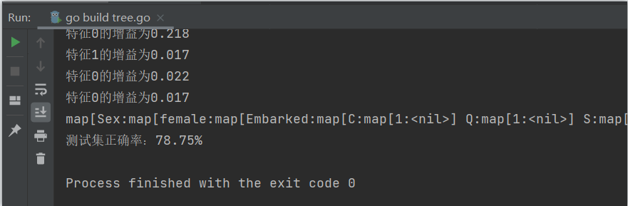
   since the accuracy of the decision tree is mainly determined by the size of the decision tree and the size of the training set, the performance of the model is evaluated by different feature sets and the proportion of the training set.
   through the experiment, the following results are obtained:

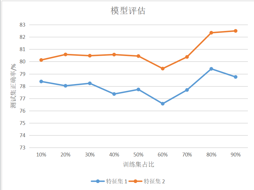
   among them, feature set 1 includes features: gender, login port; Feature set 2 contains features: gender, ticket level and landing port. Each group of experiments was run 10 times and the average value was taken.

5, Result analysis

   by analyzing the experimental results, we can find that in the case of the same feature set, the weight of the training set has little impact on the prediction accuracy of the model and will fluctuate, but the general trend is increasing, and there will be a large fluctuation when the training set accounts for 60%; When the proportion of training sets is the same, the more low correlation features, the more accurate the prediction accuracy of the model will be.