reference material:
- Rafael C. Gonzalez, Richard E. Woods, digital image processing (Third Edition) 4.11, Supporting book resources
- Alan V.Oppenheim, Ronald W.Schafer, discrete time signal processing (Third Edition) 9.5
- SPRUEB8B - TMS320C64x+ DSP Little-Endian DSP Library Programmer's Reference
- CCS Doc, 7.8 Image Analyzer
Introduction to FFT principle
the calculation of FFT must be mentioned in any book "digital signal processing". I read the book "discrete time signal processing". The whole chapter 9 introduces DFT and FFT in detail.
The recursive algorithm of the sequence of DFT is introduced to calculate the corresponding value of the sequence of DFT. Although the amount of computation of this algorithm is still proportional to
N
2
N^2
N2, but also reduces the computational complexity to a certain extent.
the later FFT algorithms of time extraction and frequency extraction are later reduced to a more general FFT algorithm in which N is a composite number. The algorithm of extracting by time is better understood. A digital sequence is divided into two sequences according to the parity of the label. It is very convenient to calculate the DFT of the whole sequence from their results. The symmetry and periodicity of the rotation factor can be flexibly used, and finally expressed as a "butterfly operation".
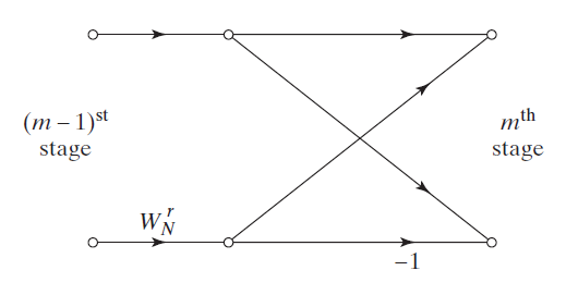
in the calculation of FFT, data storage is also an issue that needs careful consideration. If the data indexes at both ends of the butterfly operation do not need to be changed, the calculation results can be saved back to the original location without additional space. This is called "in place". After observation, it can be found that if the input is in place order, then the result calculated with the same address is positive order; If the input is in positive order, the result obtained by using the same address calculation is in place order. There are also algorithms where the input and output are in positive order, so the same address calculation is not used.
the familiar FFT algorithm, which divides the sequence into odd and even sequences for recursive operation, requires that the sequence length is a power of 2. This algorithm is called "radix-2" algorithm; If the whole sequence is divided into four groups according to a similar method, namely x[4n], x[4n+1], x[4n+2], x[4n+3], this is called "radix-4" algorithm. The number of stages required for that(
l
o
g
4
N
log_4N
log4 (N) is less, and the length of the sequence is required to be a power of 4. Of course, there is a combination of the two algorithms, mainly using radix-4, and finally using radix-2 or radix-4 according to the situation.
DSPLib configuration
it doesn't matter where the DSP library is installed. You can find the installed DSP library on the window - > Preferences - > Code Composer Studio - > Products page.
but I don't know how to use this product. Even if I check this product in the actual project, it doesn't seem to be useful.
when running the routine, I saw that the source file only contained dsplib h. So just include its path and the corresponding static library.
you can add the installation path of DSP under window - > Preferences - > Code Composer Studio - > build - > environment page. It is convenient to set the corresponding included path and included static library in the project.
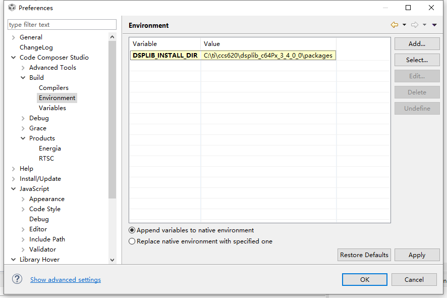
Image data generation
read the image data with OpenCV python, adjust the image resolution, scale the length and width in the same proportion, and fill "0" in the blank area to meet the requirements of FFT for the integer power of 2. Generate output h file and image after resolution adjustment.
import cv2

img = cv2.imread("Fig0431(d)(blown_ic_crop).tif",cv2.IMREAD_GRAYSCALE)
fp_code = open('..\\FFT2\\image.h','w') #the path should adjust as your need

# the destinate image size
dst_height = 1024
dst_width = 1024

# the image size of raw image
height = img.shape[0]
width = img.shape[1]

#calculate the scale
scale = min(dst_height/height,dst_width/width)

#resize the image, using the same scale for both width and height
res = cv2.resize(img, None, fx=scale, fy=scale,interpolation=cv2.INTER_AREA)

#fill the reigon where is blank with black
res = cv2.copyMakeBorder(res,0,round(dst_height-height*scale), 0, round(dst_width-width*scale),cv2.BORDER_CONSTANT,value=[0])

# write data to .h file
linestride = int(dst_width/4)
fp_code.write('#pragma DATA_ALIGN(img_src, 8);\n')
fp_code.write('int img_src[] = {\n    ')
for i in range(dst_height):
    for k in range(4):
        for j in range(linestride):
            if(i==dst_height-1 and k == 3 and j == linestride-1):
                fp_code.write(str(res[i][k*linestride+j]) + ', 0')
            else:
                fp_code.write(str(res[i][k*linestride+j]) + ', 0, ')
        fp_code.write('\n    ')
fp_code.write('};\n')

# write image
cv2.imwrite("img.png",res)
FFT and IFFT in DSPLib
the functions in dsplib can be understood from the comments in the source file, or you can directly see the document SPRUEB8B. FFT is also divided into many types according to the bit width of input and output data. What I realize is that the input and output are 32-bit FFT without scaling factor, that is, the DSP under the "dsplib installation path \ packages\ti\dsplib\src" path_ Fft32x32 and DSP_ifft32x32.
under the above path, there are four folders of test routines and three implementation methods of FFT, namely pure C language implementation (_cn), C language implementation with compiler instructions (_i) and assembly implementation (_sa). Among the three methods, the code directly implemented by assembly is the most efficient and fastest. The DSP library calls the assembled FFT by default.
the calculation methods used in these three implementation methods are the same, but using special assembly instructions has higher efficiency. So if you want to understand this code, you can look at it directly_ cn version. The schematic diagram of butterfly operation is roughly as follows:
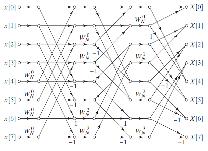
the input and output are positive sequence, and there is no same address calculation. Using the radix-4 algorithm, a butterfly operation requires four numbers. In the first level operation, the label interval of these four numbers is N/4 (radix-2 in the analogy diagram is N/2), which is represented by the variable stripe in the code, and the subsequent levels are reduced step by step.
The calculation of IFFT is very similar to FFT. We can calculate IFFT in a similar way. The calculation method is given in 4.11.2 of digital image processing.
N
x
∗
[
n
]
=
∑
n
=
0
N
−
1
X
∗
[
k
]
e
−
j
2
π
k
n
/
N
N{x^*}[n] = \sum\limits_{n = 0}^{N - 1} {{X^*}[k]{e^{ - j2\pi kn/N}}}
Nx∗[n]=n=0∑N−1X∗[k]e−j2πkn/N
generally
x
∗
[
n
]
=
x
[
n
]
x^*[n]=x[n]
X * [n]=x[n], so we only need to take the conjugate of the original complex sequence and do DFT, and then divide the result by "N" to get the result of IFFT.
Implementation of two-dimensional FFT and IFFT
the separability of two-dimensional DFT is introduced in 4.11.1 of digital image processing, that is, to realize two-dimensional DFT, DFT can be made for the two dimensions of row and column respectively. When implemented in the code, you can first do FFT on the line, then transpose the result, then do FFT on the line, and finally transpose back to get the corresponding two-dimensional DFT result\
/*
 * @func	fft2, because of transpose function, this function can be only used when width is equal to height!!!
 *
 * @param	w	=	twiddle factors
 * @param	psrc	=	source pointer, point to the image data to be processed
 * @param	ptmp	=	a pointer point to a data space, witch size is as same as the source image, just for temporary use
 * @param	width	=	image width
 * @param	height	=	image height
 */
void DSP_fft2(int *w, int *psrc, int *ptmp, int width, int height){
    int *ps = psrc;
    int *pd = ptmp;
    int i;

    // fft for the row
    for(i=0;i<height;i++){
        DSP_fft32x32(w, width, ps, pd);
        ps = ps + 2*width;
        pd = pd + 2*width;
    }

    //transpose
    transpose(ptmp, width, height);

    //fft for the column
    ps = ptmp;
    pd = psrc;
    for(i=0;i<width;i++){
        DSP_fft32x32(w, width, ps, pd);
        ps = ps + 2*width;
        pd = pd + 2*width;
    }

    //transpose
    transpose(psrc, width, height);
}
the transpose here is a general transpose, not a conjugate transpose. If the row and column lengths of the image are equal, transpose only needs to exchange the data of two positions relative to the row and column coordinates. If the length of the rows and columns of the image is not equal, additional space needs to be opened up to store the transposed data, and the additional storage overhead is large. Therefore, I didn't write this part of the code, but required the image rows and columns to be the same length.
the IFFT provided in the DSP library is only slightly modified on the basis of FFT, and some symbols are changed to realize the calculation of complex conjugate, but it is not divided by the sequence length. So every time you call DSP_ After ifft32x32, the result needs to be divided by "N" to be the result of IFFT.
/*
 * @func	ifft2, because of transpose function, this function can be only used when width is equal to height!!!
 *
 * @param	w		=	twiddle factors
 * @param	psrc	=	source pointer, point to the image data to be processed
 * @param	ptmp	=	a pointer point to a data space, witch size is as same as the source image, just for temporary use
 * @param	width	=	image width
 * @param	height	=	image height
 */
void DSP_ifft2(int *w, int *psrc, int *ptmp, int width, int height){
	int *ps = psrc;
	int *pd = ptmp;
	int i;

	//ifft for the row
	for(i=0;i<height;i++){
		DSP_ifft32x32(w, width, ps, pd);
		ps = ps + 2*width;
		pd = pd + 2*width;
	}
	for(i=0;i<2*width*height;i++){
		ptmp[i] = ptmp[i]/width;
	}

	//transpose
	transpose(ptmp, width, height);

	//ifft for the column
	ps = ptmp;
	pd = psrc;
	for(i=0;i<width;i++){
		DSP_ifft32x32(w, width, ps, pd);
		ps = ps + 2*width;
		pd = pd + 2*width;
	}
	for(i=0;i<2*width*height;i++){
		psrc[i] = psrc[i]/width;
	}

	//transpose
	transpose(psrc, width, height);
}
Image Analyzer
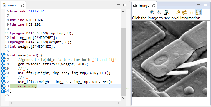
CCS has its own Image analysis tool. In the debugging interface, open tools - > Image analyzer to edit the Properties in the Properties window.
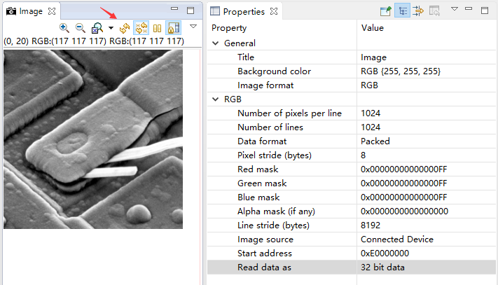
- Image Format: input the Image Format, depending on the specific data format
- Number of pixels per line
- Number of lines: number of image lines
- Data format: data format. packed means that the data of a pixel is stored continuously. Another kind of planar means that the data of the same channel is stored continuously
- Pixel stripe (bytes): pixel step, that is, how many bytes each pixel occupies
- Red/Green/Blue/Alpha mask: "1" is valid. It allows ARGB to find the value of the corresponding position from a few bytes and can overlap. The overlap of three RGB channels is a gray image.
- Line stripe (bytes): how many bytes does each line occupy
- Start address: image start address
- Read data as: format of read data, set according to the data format of image, int(32bit), short(16bit), char(8bit)
- Start address: image start address
- Read data as: format of read data, set according to the data format of image, int(32bit), short(16bit), char(8bit)
after setting, click the refresh button in the Image window to refresh the displayed Image.
test result
pre stored image:
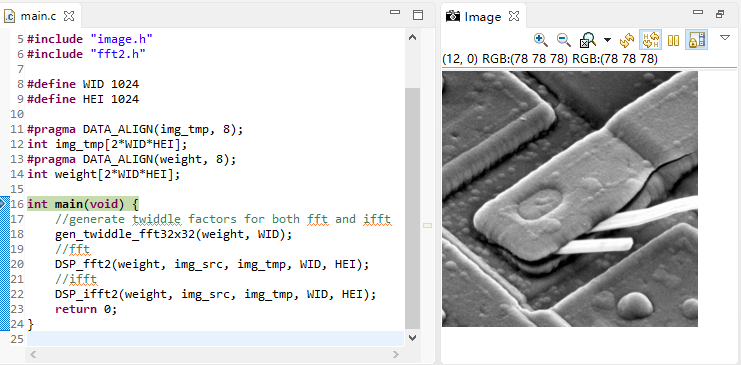
after FFT transformation, the actual data has exceeded the gray range and cannot display the normal FFT spectrum:
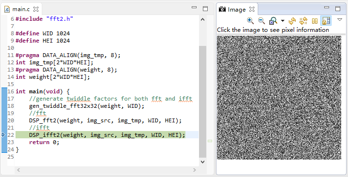
IFFT transformed image:
