1 logistic growth model
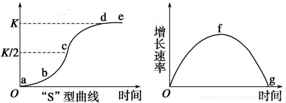
1.1 J-type growth and S-type growth
Exponential growth, J-shaped curve: exponential growth, that is, the growth is not restrained and explosive.
For example, one person can infect three people, three people can infect nine people, and nine people can infect 27 people, which keeps doubling. This is J-type growth, also known as exponential growth.
Some infectious diseases may show exponential growth in the initial stage.
However, in the actual growth process, the growth rate cannot be maintained all the time. With the increasing number of people, the growth rate will be gradually restrained. This is S-type growth.
The spread of general diseases is an S-type growth process, because there will be some resistance in the process of disease transmission.
1.2 logistic growth function
When a species moves into a new ecosystem, its number will change. Assuming that the initial number of the species is less than the maximum capacity of the environment, the number will increase. If the species has natural enemies, food, space and other resources in this ecosystem and is also insufficient (non ideal environment), the growth function meets the logistic equation, and the image is S-shaped. This equation is the best mathematical model to describe the law of population growth under the condition of limited resources. In the following contents, the principle, ecological significance and application of logistic equation will be introduced in detail. The differential formula of logistic model is: dx/dt=rx(1-x), in which r is the rate parameter.
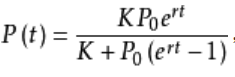
- K is the environmental capacity, that is, the limit that P(t) can reach when it grows to the end.
- P0 is the initial capacity, which is the number at t=0.
- r is the growth rate. The larger r is, the faster it will grow and approach the value of K. The smaller r is, the slower it will grow and approach the value of K.
The formula is written in python in the form of function:
def logistic_increase_function(t,K,P0,r):
    # t:time   t0:initial time    P0:initial_value    K:capacity  r:increase_rate
    exp_value=np.exp(r*(t-t0))
    return (K*exp_value*P0)/(K+(exp_value-1)*P0)
The curve of logistic growth is also called s-shaped curve. The figure below shows the number of curves on the left and the growth rate on the right.
1.3 case code
#!/usr/bin/python
# -*- coding: UTF-8 -*-
"""
Fitting 2019-nCov Number of confirmed pneumonia infections
"""
import numpy as np
import matplotlib.pyplot as plt
import math
import pandas as pd
import numpy as np
import matplotlib.pyplot as plt
from scipy.optimize import curve_fit
def logistic_increase_function(t,K,P0,r):
'''
t ,list,Date series,[11,18,19,20 ,21, 22, 23, 24, 25, 26, 27]
t0,int,Date first day
r,float,r Is the growth rate, r The larger, the faster the growth, the faster the approach K value - Steeper;r The smaller, the slower the growth, the slower the approach K Value.
P0 Is the initial capacity, which is t=0 Number of moments
K,float,K Is the environmental capacity, that is, to grow to the end, P(t)The limit that can be reached,Generally 1
'''
t0=11 # first day
r=0.6
# r = 0.55
# t:time t0:initial time P0:initial_value K:capacity r:increase_rate
exp_value=np.exp(r*(t-t0))
return (K*exp_value*P0)/(K+(exp_value-1)*P0)
'''
1.11 41 cases per day
1.18 45 cases per day
1.19 62 cases per day
1.20 291 cases per day
1.21 440 cases per day
1.22 571 cases per day
1.23 830 cases per day
1.24 1287 cases per day
1.25 1975 cases in Japan
1.26 2744 cases per day
1.27 4515 cases per day
'''
# Date and number of infected persons
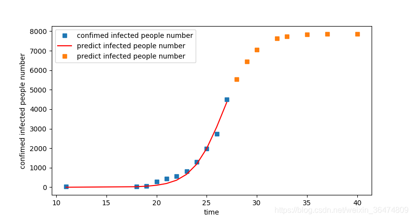
t=[11,18,19,20 ,21, 22, 23, 24, 25, 26, 27]
t=np.array(t)
P=[41,45,62,291,440,571,830,1287,1975,2744,4515]
P=np.array(P)
# Estimation and fitting by least square method
popt, pcov = curve_fit(logistic_increase_function, t, P)
# popt - K,P0,r
# Finally, K=4.01665705e+10 people will be infected
# array([7.86278276e+03, 2.96673434e-01, 1.00000000e+00])
#Get the fitting coefficient in popt
print("K:capacity P0:initial_value r:increase_rate t:time")
print(popt)
#Predicted P value after fitting
P_predict = logistic_increase_function(t,popt[0],popt[1],popt[2])
#Future forecast
future=[11,18,19,20 ,21, 22, 23, 24, 25, 26, 27,28,29,30,31,41,51,61,71,81,91,101]
future=np.array(future)
future_predict=logistic_increase_function(future,popt[0],popt[1],popt[2])
#Recent situation forecast
tomorrow=[28,29,30,32,33,35,37,40]
tomorrow=np.array(tomorrow)
tomorrow_predict=logistic_increase_function(tomorrow,popt[0],popt[1],popt[2])
#mapping
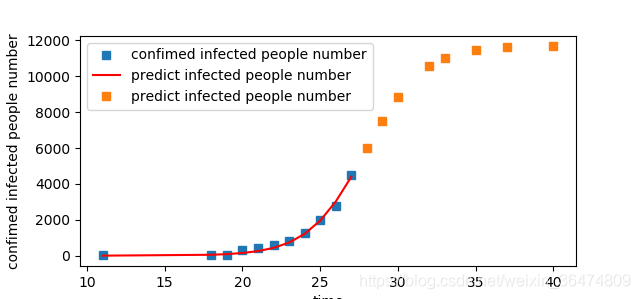
plot1 = plt.plot(t, P, 's',label="confimed infected people number")
plot2 = plt.plot(t, P_predict, 'r',label='predict infected people number')
plot3 = plt.plot(tomorrow, tomorrow_predict, 's',label='predict infected people number')
plt.xlabel('time')
plt.ylabel('confimed infected people number')
plt.legend(loc=0) #Specify the lower right corner of the position of legend
print(logistic_increase_function(np.array(28),popt[0],popt[1],popt[2]))
print(logistic_increase_function(np.array(29),popt[0],popt[1],popt[2]))
plt.show()
#Future forecast mapping
#plot2 = plt.plot(t, P_predict, 'r',label='polyfit values')
#plot3 = plt.plot(future, future_predict, 'r',label='polyfit values')
#plt.show()
print("Program done!")
'''
# Fitting age
'''
import numpy as np
import matplotlib.pyplot as plt
#Define x and y scatter coordinates
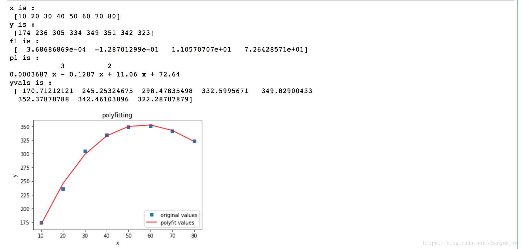
x = [10,20,30,40,50,60,70,80]
x = np.array(x)
print('x is :\n',x)
num = [174,236,305,334,349,351,342,323]
y = np.array(num)
print('y is :\n',y)
#Fitting with cubic polynomial
f1 = np.polyfit(x, y, 3)
print('f1 is :\n',f1)
p1 = np.poly1d(f1)
print('p1 is :\n',p1)
#You can also use yvals = NP polyval(f1, x)
yvals = p1(x)
print('yvals is :\n',yvals)
#mapping
plot1 = plt.plot(x, y, 's',label='original values')
plot2 = plt.plot(x, yvals, 'r',label='polyfit values')
plt.xlabel('x')
plt.ylabel('y')
plt.legend(loc=4) #Specify the position of the lower right corner of the legend
plt.title('polyfitting')
plt.show()
The least square method is used for fitting, and the least square method is used to fit the logistic growth function.
logistic_ increase_ The value of r in function (T, K, P0, r) can be adjusted:
After human intervention, the disease reduces the K value, so the r value can be increased to speed up the speed of reaching the K value
(r becomes larger and the curve becomes steeper)
r = 0.55
r=0.65
2 fitting polynomial function
reference resources: Three schemes of quasi merging arbitrary data and curves to obtain function expression in python.
2.1 polynomial fitting - polyfit fitting age
import numpy as np
import matplotlib.pyplot as plt

#Define x and y scatter coordinates
x = [10,20,30,40,50,60,70,80]
x = np.array(x)
print('x is :\n',x)
num = [174,236,305,334,349,351,342,323]
y = np.array(num)
print('y is :\n',y)
#Fitting with cubic polynomial
f1 = np.polyfit(x, y, 3)
print('f1 is :\n',f1)

p1 = np.poly1d(f1)
print('p1 is :\n',p1)

#You can also use yvals = NP polyval(f1, x)
yvals = p1(x)  #Fitting y value
print('yvals is :\n',yvals)
#mapping
plot1 = plt.plot(x, y, 's',label='original values')
plot2 = plt.plot(x, yvals, 'r',label='polyfit values')
plt.xlabel('x')
plt.ylabel('y')
plt.legend(loc=4) #Specify the lower right corner of the position of legend
plt.title('polyfitting')
plt.show()
2.2 polynomial fitting - curve_fit polynomial
import numpy as np
import matplotlib.pyplot as plt
from scipy.optimize import curve_fit
#Custom function e exponential form
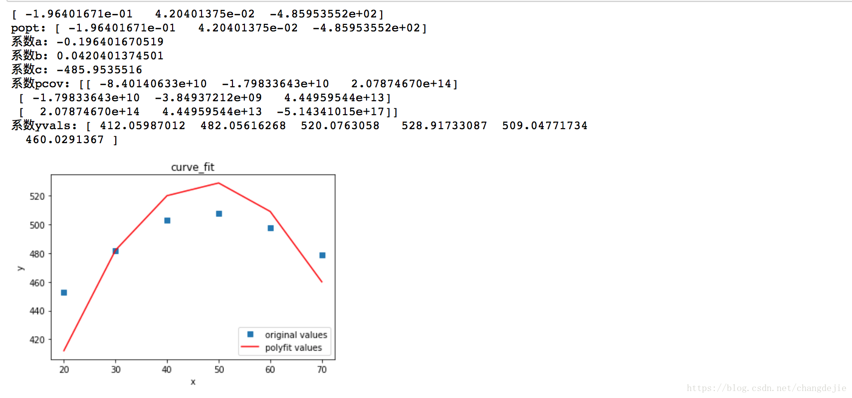
def func(x, a, b,c):
return a*np.sqrt(x)*(b*np.square(x)+c)
#Define x and y scatter coordinates
x = [20,30,40,50,60,70]
x = np.array(x)
num = [453,482,503,508,498,479]
y = np.array(num)
#Nonlinear least square fitting
popt, pcov = curve_fit(func, x, y)
#Get the fitting coefficient in popt
print(popt)
a = popt[0]
b = popt[1]
c = popt[2]
yvals = func(x,a,b,c) #y value fitting
print('popt:', popt)
print('coefficient a:', a)
print('coefficient b:', b)
print('coefficient c:', c)
print('coefficient pcov:', pcov)
print('coefficient yvals:', yvals)
#mapping
plot1 = plt.plot(x, y, 's',label='original values')
plot2 = plt.plot(x, yvals, 'r',label='polyfit values')
plt.xlabel('x')
plt.ylabel('y')
plt.legend(loc=4) #Specify the lower right corner of the position of legend
plt.title('curve_fit')
plt.show()
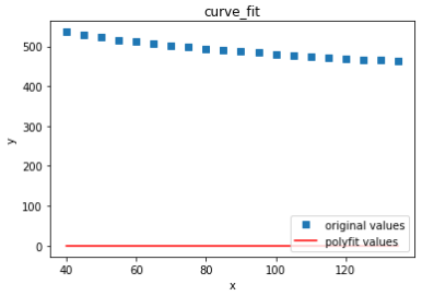
2.3 curve_fit fitting Gaussian distribution
#encoding=utf-8
import numpy as np
import matplotlib.pyplot as plt
from scipy.optimize import curve_fit
import pandas as pd

#Custom function e exponential form
def func(x, a,u, sig):
    return  a*(np.exp(-(x - u) ** 2 /(2* sig **2))/(math.sqrt(2*math.pi)*sig))*(431+(4750/x))


#Define x and y scatter coordinates
x = [40,45,50,55,60,65,70,75,80,85,90,95,100,105,110,115,120,125,130,135]
x=np.array(x)
# x = np.array(range(20))
print('x is :\n',x)
num = [536,529,522,516,511,506,502,498,494,490,487,484,481,478,475,472,470,467,465,463]
y = np.array(num)
print('y is :\n',y)

popt, pcov = curve_fit(func, x, y,p0=[3.1,4.2,3.3])
#Get the fitting coefficient in popt
a = popt[0]
u = popt[1]
sig = popt[2]


yvals = func(x,a,u,sig) #Fitting y value
print(u'coefficient a:', a)
print(u'coefficient u:', u)
print(u'coefficient sig:', sig)

#mapping
plot1 = plt.plot(x, y, 's',label='original values')
plot2 = plt.plot(x, yvals, 'r',label='polyfit values')
plt.xlabel('x')
plt.ylabel('y')
plt.legend(loc=4) #Specify the lower right corner of the position of legend
plt.title('curve_fit')
plt.show()