Chapter 1 construction of experimental environment
This chapter will mainly introduce anaconda and Jupyter Notebook. Including how to install Anaconda on windows, Mac, linux and other platforms, as well as the basic startup and use methods of Jupyter Notebook.
1-1 guidance video
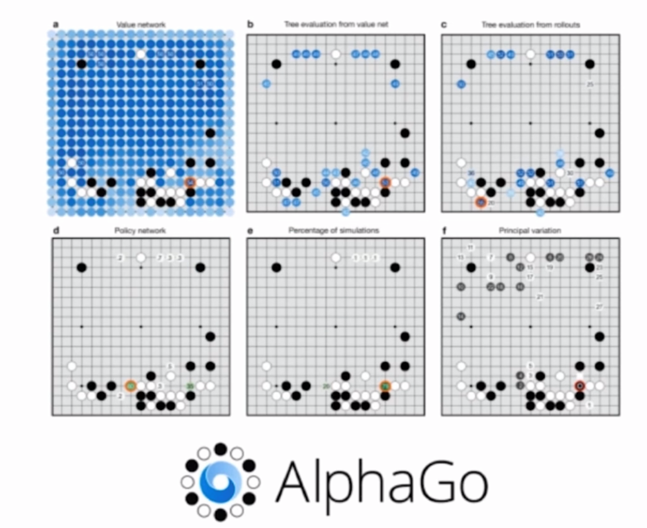
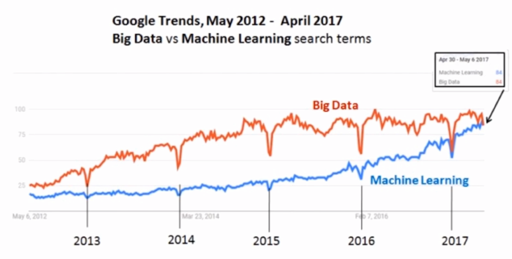
Mathematical science and machine learning


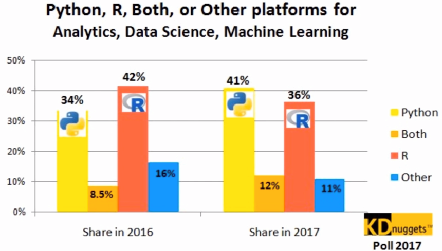
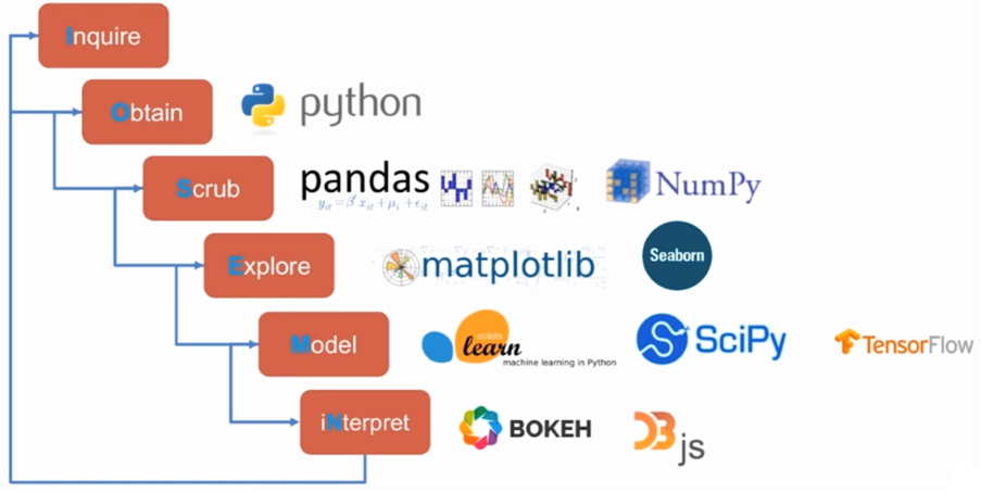
Mathematical science workflow
Specific course arrangement:
- Chapter 1: Construction of experimental environment
- Chapter 2: introduction to Numpy
- Chapter 3: introduction to Pandas
- Chapter 4: Pandas play data
- Chapter 5: drawing and visualization - Matplotlib
- Chapter 6: drawing and visualization Seaborn
- Chapter 7: actual combat of data analysis project
- Chapter 8: summary
Suitable for people:
- Have certain self-study and practical ability
- Have the most basic Python Foundation
- I want to work in data analysis and machine learning related fields in the future
1-2 introduction to anaconda and Jupyter notebook
Anaconda/Jupyter notebook: open Data Science Platform
What is Anaconda?

- The most famous Python data science platform
- 750 + popular Python & R packages
- Cross platform: Windows, Mac, Linux
- conda: Extensible package management tool
- Free distribution
- A very active community
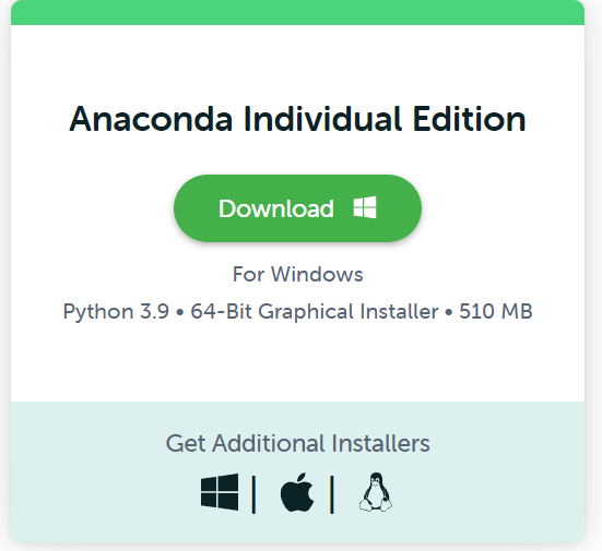
Installation of Anaconda
Download address
- Now? https://www.anaconda.com/products/individual
- Before: https://www.anaconda.com/download/
Check for correct installation:
cd ~/anaconda
bin/conda --version
conda 4.3.21
Conda: Package and Environment management
- Install Packages
- Update Packages
- Create sandbox: Conda environment
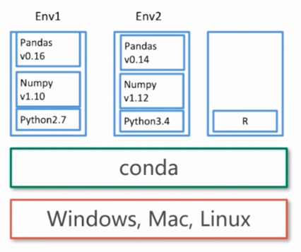
Conda's Environment management
Create a new environment
conda create --name python34 python3.4
Activate an environment
activate python34 # for Windows
source activate python34 # for Linux & Mac
Exit an environment
deactivate python34 # for Windows
source deactivate python34 # for Linux & Mac
Delete an environment
conda remove --name python34 --all
package management of Conda
Conda's package management is a bit like pip
Install a Python package
conda install numpy
View installed Python packages
conda list
conda list -n python34 #View Python packages installed in the specified environment
Delete a Python package
conda remove --name python34 numpy
Data Science IDE vs Developer IDE
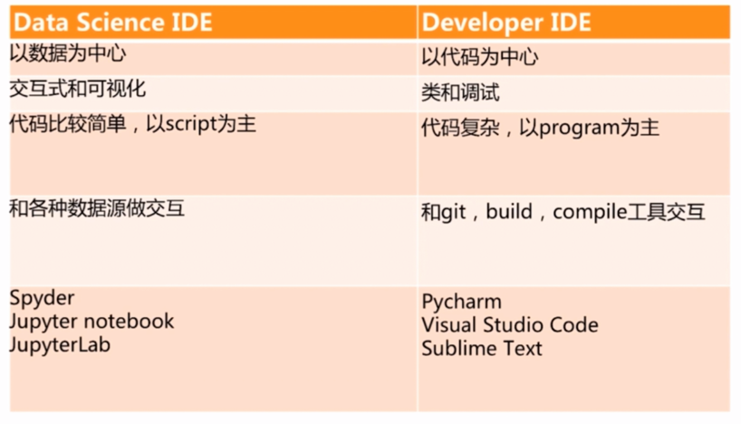
Data Science IDEs in Anaconda
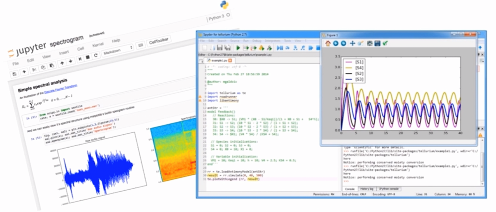
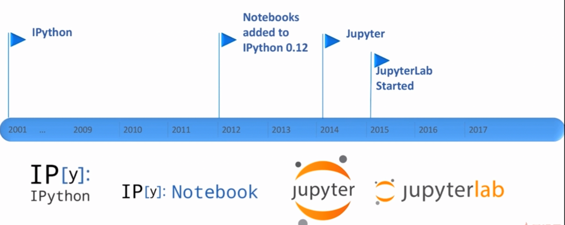
From IPython to Jupyter
What is Ipython?

- A powerful interactive shell
- It's Jupyter's kernel
- Support interactive data analysis and visualization
Ipython Kernel
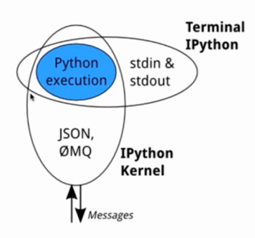
- Mainly responsible for running user code
- Interact with the python shell through stdin/stdout
- Interact with ZeroMQ and notebook with json message
What is Jupyter Notebook?

- Formerly known as Ipython notebook
- An open source Web application
- You can create and share documents that contain code, views, and comments
- It can be used in data statistics, analysis, modeling, machine learning and other fields
Interaction between Notebook and kernel
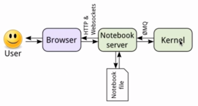
- The core is Notebook server
- Server save and notebook load
File format (. ipynb) of Notebook
- A format defined by IPython Notebook (json)
- You can read online data, CSV/XLS files
- It can be converted to other formats (py,html,pdf,md, etc.)
NBViewer

- An online ipynb format notebook presentation tool
- Can be shared via url
- Github integrates NBViewer
- Easily integrate into blogs, emails, Wikis and Books through converter
Laboratory environment of this course
- Installing Anaconda on Windows/Mac/Linux
- Use Python 3 6 as the basic environment
- Using Jupiter notebook as the programming IDE
1-3 installation demonstration of Anaconda on Mac
Download the macOS version installation package, python 3 6 + 64 bit version (as of February 15, 2022, python 3.9)
Anaconda3-2021.11-MacOSX-x86_64.pkg
Select Install for me only for other basic default options
It is not recommended to change the installation directory (1.44gb is required for installation)
~] ls
~] pwd
~] cd anaconda/
anaconda] ls
anaconda] cd bin
bin] ./conda --version
conda 4.3.21
bin] ./conda list
bin] ./jupyter notebook # Open browser
1-4 Anaconda installation demonstration on windows
Download the Windows version installation package, python 3 6 + 64 bit version (as of February 15, 2022, python 3.9)
Anaconda3-2021.11-Windows-x86_64.exe
Select Just Me(recommended) and other basic default options
The installed Anaconda3 can be seen in the [Start Menu]
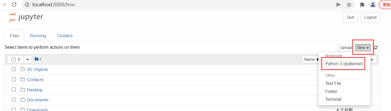
Open Jupiter notebook
1-5 installation demonstration of Anaconda on Linux
Download the Linux version installation package, python 3 6 + 64 bit version (as of February 15, 2022, python 3.9)
Copy installation package link
~] wget https://repo.anaconda.com/archive/Anaconda3-2021.11-Linux-x86_64.sh
~] ls
Anaconda3-2021.11-Linux-x86_64.sh
~] ls -lh
~] sh Anaconda3-2021.11-Linux-x86_64.sh # Select Default Options
~] pwd
/home/centos
~] cd anaconda3
anaconda3] ls
anaconda3] cd bin
anaconda3] ./conda --version
conda 4.3.21
anaconda3] ./jupyter notebook --no-browser # Copy link
Local terminal
~ ssh -N -f -L localhost:888:localhost:8888 gitlab-demo-ci
~ ssh -N -f -L localhost:888:localhost:8888 root@gitlab-demo-ci
The browser opens and the link is copied in
!ifconfig # Corresponding to ifconfig in linux system
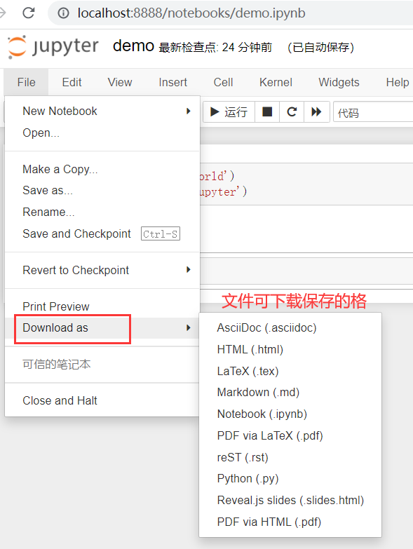
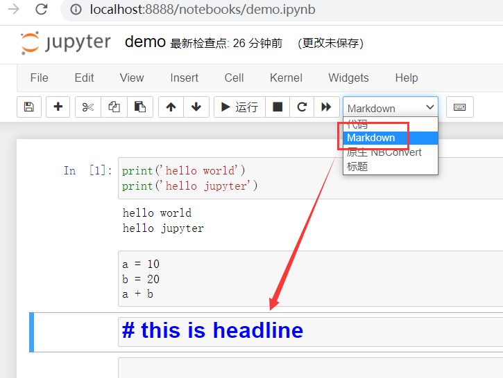
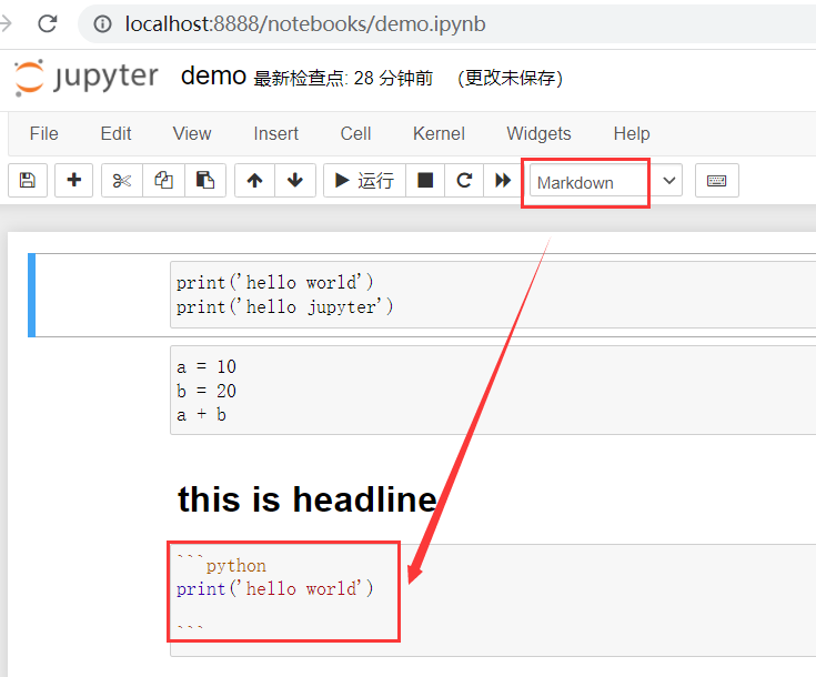
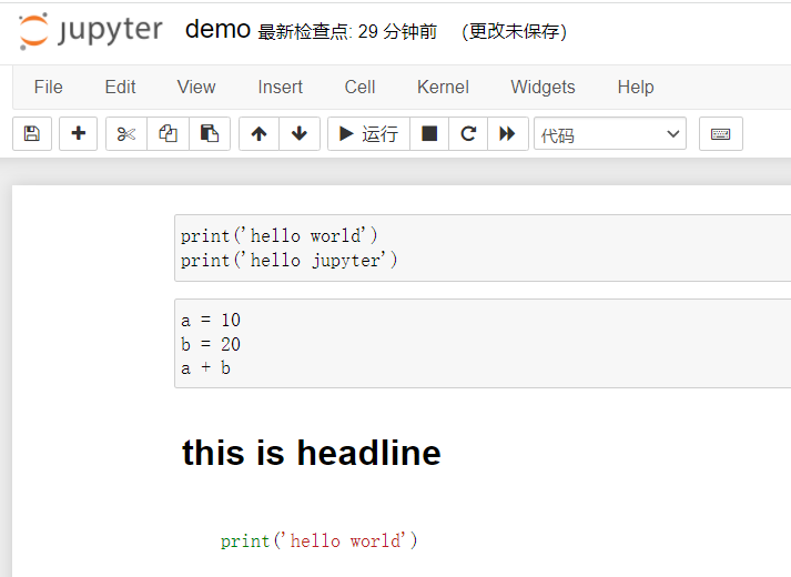
1-6 demonstration of using Jupiter notebook
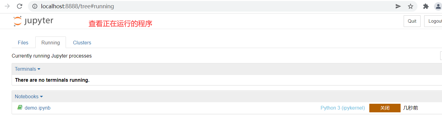
cd anaconda3
cd jupyter-notebook/python-data-science
python-data-science git:(master) ls
README.md    demo.ipynb
python-data-science git:(master) xx/bin/jupyter notebook # Openable
Chapter 2 Introduction to Numpy
This chapter will introduce Numpy, the most basic library in the field of Python data science, review the basis of matrix operation, introduce the most important data structure Array and how to perform Array and matrix operation through Numpy.
2-1 five commonly used Python libraries in the field of data science
- Numpy
- Scipy
- Pandas
- Matplotlib
- Scikit-learn
Numpy
- N-dimensional array (matrix), fast and efficient, vector attribute operation
- Efficient Index without loop
- Open source, free cross platform, and its operation efficiency is comparable to that of C/Matlab
Scipy
- Rely on Numpy
- Designed for science and Engineering
- A variety of commonly used scientific calculations are realized: linear algebra, Fourier transform, signal and image processing
Pandas
- Structured data analysis tool (relying on Numpy)
- It provides a variety of advanced data structures: time series, DataFrame and Panel
- Strong data indexing and processing capabilities
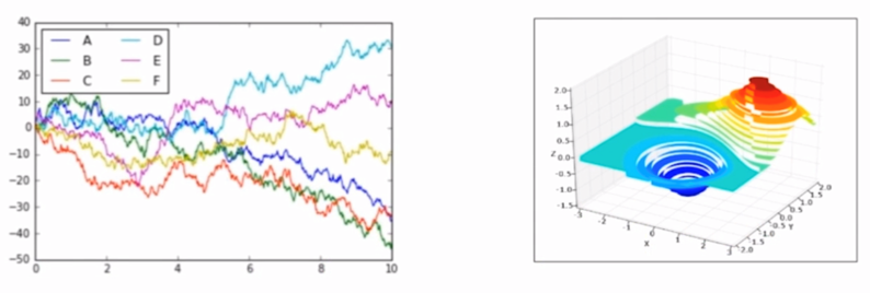
Matplotlib
- Python is the most widely used suite in 2D drawing
- It can basically replace the drawing function of Matlab (scatter, curve, column, etc.)
- You can draw exquisite 3D pictures through mplot3d
Scikit-learn
- Python module of machine learning
- Based on Scipy, it provides common machine learning algorithms: clustering and regression
- Easy to learn API interface

2-2 matrix operation of basic review of Mathematics
Basic concepts
- Matrix: rectangular data, that is, a two-dimensional array. Vector and scalar are special cases of matrix
- Vector: refers to the matrix of 1xn or nx1
- Scalar: 1x1 matrix
- When the array of N dimensions is extended
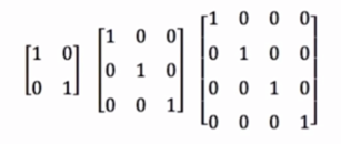
Special matrix
- All 0 and all 1 matrices
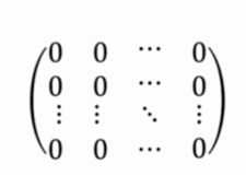
- Identity matrix
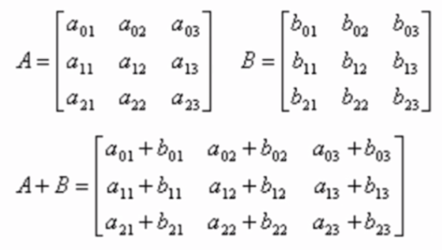
Matrix addition and subtraction
- The two matrices of addition and subtraction must have the same row and column
- Addition and subtraction of corresponding elements of row and column
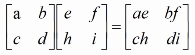
Array multiplication (dot multiplication)
- Array multiplication (dot multiplication) is the multiplication between corresponding elements
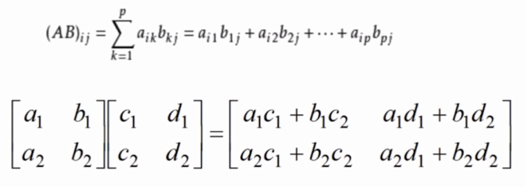
Matrix multiplication
Let A be the matrix of mxp, B be the matrix of pxn, and matrix C of mxn be the product of A and B, denoted as C=AB, where the elements in row i and column j of matrix C can be expressed as:
Other knowledge of linear algebra
- Linear algebra published by Tsinghua University
- http://bs.szu.edu.cn/sljr/Up/day_110824/201108240409437708.pdf
2-3 creation and access of array
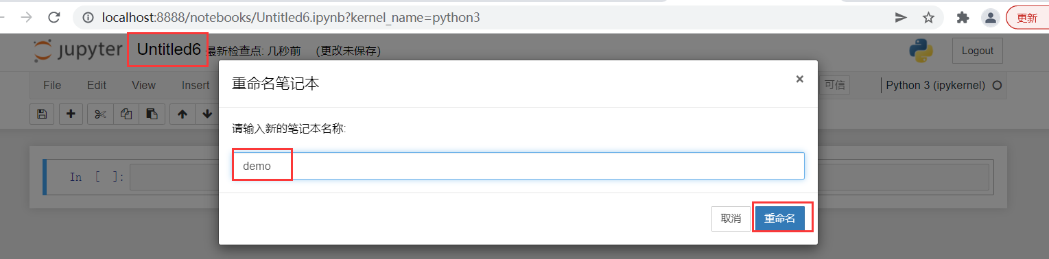
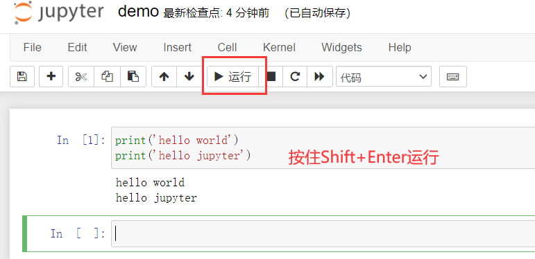
Jupyter notebook creates a new file array ipynb
# Creation and access of arrays
import numpy as np
# create from python list
list_1 = [1, 2, 3, 4]
list_1        #  [1, 2, 3, 4]
array_1 = np.array(list_1)
array_1        # array([1, 2, 3, 4])
list_2 = [5, 6, 7, 8]
array_2 = np.array([list_1,list_2])
array_2
# array([[1, 2, 3, 4],
       [5, 6, 7, 8]])
array_2.shape    # (2, 4)
array_2.size    # 8
array_2.dtype    # dtype('int32 ') look at the computer, or dtype('int64')
array_3 = np.array([[1.0,2,3],[4.0,5,6]])
array_3.dtype        # dtype('float64')
array_4 = np.arange(1,10)
array_4        # array([1, 2, 3, 4, 5, 6, 7, 8, 9])
array_4 = np.arange(1, 10, 2)
array_4        # array([1, 3, 5, 7, 9])
np.zeros(5)        # array([0., 0., 0., 0., 0.])    # Zero matrix
np.zeros([2,3])        # Two dimensional zero matrix with two rows and three columns
# array([[0., 0., 0.],
       [0., 0., 0.]])
np.eye(5)    # Identity matrix with n=5
# array([[1., 0., 0., 0., 0.],
       [0., 1., 0., 0., 0.],
       [0., 0., 1., 0., 0.],
       [0., 0., 0., 1., 0.],
       [0., 0., 0., 0., 1.]])
np.eye(5).dtype        # dtype('float64')
a = np.arange(1,10)
a        # array([1, 2, 3, 4, 5, 6, 7, 8, 9])
a[1]    # 2 (take the second element of the array)
a[1:5]    # array([2, 3, 4, 5]) takes the 2nd-5th element of the array
b = np.array([[1,2,3],[4,5,6]])
b
# array([[1, 2, 3],
       [4, 5, 6]])
b[1][0]        # 4
b[1,0]        # 4
c = np.array([[1,2,3],[4,5,6],[7,8,9]])
c
# array([[1, 2, 3],
       [4, 5, 6],
       [7, 8, 9]])
c[:2,1:]
# array([[2, 3],
       [5, 6]])
2-4 array and matrix operation
Jupyter notebook creates a new file array and matrix operation ipynb
# Quickly create an array
import numpy as np
np.random.randn(10)        # Returns a one-dimensional array of 10 decimal elements
# array([ 0.26674666, -0.91111093,  0.30684449, -0.80206634, -0.89176532,
        0.7950014 , -0.53259808, -0.09981816,  1.2960139 , -0.9668373 ])
np.random.randint(10)    # 0
np.random.randint(10,size=(2,3))    # Generate a 2x3 two-dimensional array with array elements [0,9]
# array([[7, 5, 8],
       [1, 5, 8]])
np.random.randint(10,size=20)        # Generate a one-dimensional array of 20 elements, array elements [0,9]
# array([5, 6, 4, 8, 0, 9, 6, 2, 2, 9, 2, 1, 4, 6, 1, 5, 8, 2, 3, 4])
np.random.randint(10,size=20).reshape(4,5)    # Reshape the one-dimensional array generating 20 elements into a 4x5 two-dimensional array, with array elements [0,9]
# array([[7, 1, 0, 5, 7],
       [8, 0, 3, 7, 9],
       [9, 0, 7, 3, 2],
       [9, 1, 5, 8, 7]])

# Array operation
a = np.random.randint(10,size=20).reshape(4,5)
b = np.random.randint(10,size=20).reshape(4,5)
a
# array([[2, 3, 8, 4, 8],
       [0, 7, 9, 9, 9],
       [1, 8, 1, 8, 6],
       [3, 4, 7, 5, 1]])
b
# array([[8, 4, 3, 1, 6],
       [4, 4, 6, 2, 9],
       [9, 4, 8, 5, 8],
       [6, 2, 5, 5, 8]])
a + b
# array([[10,  7, 11,  5, 14],
       [ 4, 11, 15, 11, 18],
       [10, 12,  9, 13, 14],
       [ 9,  6, 12, 10,  9]])
a - b
# array([[-6, -1,  5,  3,  2],
       [-4,  3,  3,  7,  0],
       [-8,  4, -7,  3, -2],
       [-3,  2,  2,  0, -7]])
a * b
# array([[16, 12, 24,  4, 48],
       [ 0, 28, 54, 18, 81],
       [ 9, 32,  8, 40, 48],
       [18,  8, 35, 25,  8]])
a / b
# An error may be reported to see if there is an element 0 in b
array([[0.25      , 0.75      , 2.66666667, 4.        , 1.33333333],
       [0.        , 1.75      , 1.5       , 4.5       , 1.        ],
       [0.11111111, 2.        , 0.125     , 1.6       , 0.75      ],
       [0.5       , 2.        , 1.4       , 1.        , 0.125     ]])
np.mat([[1,2,3],[4,5,6]])
# matrix([[1, 2, 3],
        [4, 5, 6]])
a
# array([[2, 3, 8, 4, 8],
       [0, 7, 9, 9, 9],
       [1, 8, 1, 8, 6],
       [3, 4, 7, 5, 1]])
np.mat(a)
#
matrix([[2, 3, 8, 4, 8],
        [0, 7, 9, 9, 9],
        [1, 8, 1, 8, 6],
        [3, 4, 7, 5, 1]])

# Matrix operation
A = np.mat(a)
B = np.mat(b)
A
# matrix([[2, 3, 8, 4, 8],
        [0, 7, 9, 9, 9],
        [1, 8, 1, 8, 6],
        [3, 4, 7, 5, 1]])
B
# matrix([[8, 4, 3, 1, 6],
        [4, 4, 6, 2, 9],
        [9, 4, 8, 5, 8],
        [6, 2, 5, 5, 8]])
A + B
# matrix([[10,  7, 11,  5, 14],
        [ 4, 11, 15, 11, 18],
        [10, 12,  9, 13, 14],
        [ 9,  6, 12, 10,  9]])
A - B
# matrix([[-6, -1,  5,  3,  2],
        [-4,  3,  3,  7,  0],
        [-8,  4, -7,  3, -2],
        [-3,  2,  2,  0, -7]])
A * B    # An error is reported. The number of columns of A is inconsistent with the number of rows of B

a = np.mat(np.random.randint(10,size=20).reshape(4,5))
b = np.mat(np.random.randint(10,size=20).reshape(5,4))
a
# matrix([[9, 9, 3, 0, 5],
        [9, 4, 6, 4, 5],
        [9, 0, 7, 0, 9],
        [7, 2, 6, 0, 6]])
b
# matrix([[2, 2, 6, 4],
        [8, 9, 8, 0],
        [2, 1, 3, 9],
        [3, 1, 0, 2],
        [9, 3, 1, 4]])
a * b
# matrix([[141, 117, 140,  83],
        [119,  79, 109, 118],
        [113,  52,  84, 135],
        [ 96,  56,  82, 106]])

# Array common functions
a = np.random.randint(10,size=20).reshape(4,5)
np.unique(a)    # De duplication of all elements in a
# array([0, 1, 2, 3, 4, 5, 6, 8, 9])
a
# array([[4, 2, 8, 4, 2],
       [6, 9, 6, 4, 0],
       [9, 2, 6, 9, 0],
       [1, 3, 8, 5, 9]])
sum(a)        # Sum all rows and columns in a
# array([20, 16, 28, 22, 11])
sum(a[0])    # Sum the first line in a
# 20
sum(a[:,0])    # Sum the first column in a
# 20
a.max()        # Maximum value in a
# 9
max(a[0])    # Maximum value of the first row in a
# 8
max(a[:,0])    # Maximum value of the first column in a
# 9
2-5 input and output of array
Jupyter notebook creates a new file, input and output of Array ipynb
# Serialize numpy array using pickle
import pickle
import numpy as np
x = np.arange(10)
x
# array([0, 1, 2, 3, 4, 5, 6, 7, 8, 9])
f = open('x.pk1','wb')
pickle.dump(x, f)
!ls        # windows system is available! dir
# Array.ipynb# array input and output ipynb
  x.pk1                    Array and matrix operation.ipynb
f = open('x.pk1','rb')
pickle.load(f)
# array([0, 1, 2, 3, 4, 5, 6, 7, 8, 9])
np.save('one_array', x)
!ls
# Array.ipynb# array input and output ipynb
  x.pk1                    one_array.npy
  Array and matrix operation.ipynb
np.load('one_array.npy')
# array([0, 1, 2, 3, 4, 5, 6, 7, 8, 9])
y = np.arange(20)
y
# array([ 0,  1,  2,  3,  4,  5,  6,  7,  8,  9, 10, 11, 12, 13, 14, 15, 16,
       17, 18, 19])
np.savez('two_array.npz', a=x, b=y)
!ls
# Array.ipynb                        two_array.npz
  Array of input and output.ipynb        x.pk1
  one_array.npy                        Array and matrix operation.ipynb
np.load('two_array.npz')
# <numpy.lib.npyio.NpzFile at 0x17033c77df0>
c = np.load('two_array.npz')
c['a']
# array([0, 1, 2, 3, 4, 5, 6, 7, 8, 9])
c['b']
# array([ 0,  1,  2,  3,  4,  5,  6,  7,  8,  9, 10, 11, 12, 13, 14, 15, 16,
       17, 18, 19])
scipy document
- Now? https://docs.scipy.org/doc/scipy/getting_started.html
- Before: https://docs.scipy.org/doc/numpy-dev/user/quickstart.html
Chapter 3 Introduction to Pandas
This chapter will introduce pandas, the most important library for data analysis in the field of Python data science. We will start with the two most important data structures Series and DataFrame in pandas, introduce their creation and basic operation, and understand the relationship between Series and DataFrame through practical operation.
3-1 Pandas Series
Jupyter notebook creates a new file series ipynb
import numpy as np
import pandas as pd
s1 = pd.Series([1,2,3,4])
s1
# 0    1
  1    2
  2    3
  3    4
  dtype: int64
s1.values
# array([1, 2, 3, 4], dtype=int64)
s1.index
# RangeIndex(start=0, stop=4, step=1)
s2 = pd.Series(np.arange(10))
s2            # Some computers dtype: int64
# 0    0
  1    1
  2    2
  3    3
  4    4
  5    5
  6    6
  7    7
  8    8
  9    9
  dtype: int32
s3 = pd.Series({'1':1, '2':2, '3':3})
s3
# 1    1
  2    2
  3    3
  dtype: int64
s3.values
# array([1, 2, 3], dtype=int64)
s3.index
# Index(['1', '2', '3'], dtype='object')
s4 = pd.Series([1,2,3,4],index=['A','B','C','D'])
s4
# A    1
  B    2
  C    3
  D    4
  dtype: int64
s4.values
# array([1, 2, 3, 4], dtype=int64)
s4.index
# Index(['A', 'B', 'C', 'D'], dtype='object')
s4['A']
# 1
s4[s4>2]
# C    3
  D    4
  dtype: int64
s4
# A    1
  B    2
  C    3
  D    4
  dtype: int64
s4.to_dict()
# {'A': 1, 'B': 2, 'C': 3, 'D': 4}
s5 = pd.Series(s4.to_dict())
s5
# A    1
  B    2
  C    3
  D    4
  dtype: int64
index_1 = ['A', 'B', 'C', 'D','E']
s6 = pd.Series(s5,index=index_1)
s6
# A    1.0
  B    2.0
  C    3.0
  D    4.0
  E    NaN
  dtype: float64
pd.isnull(s6)
# A    False
  B    False
  C    False
  D    False
  E     True
dtype: bool
pd.notnull(s6)
# A     True
  B     True
  C     True
  D     True
  E    False
  dtype: bool
s6
# A    1.0
  B    2.0
  C    3.0
  D    4.0
  E    NaN
  dtype: float64
s6.name = 'demo'
s6
# A    1.0
  B    2.0
  C    3.0
  D    4.0
  E    NaN
  Name: demo, dtype: float64
s6.index.name = 'demo index'
s6
# demo index
  A    1.0
  B    2.0
  C    3.0
  D    4.0
  E    NaN
  Name: demo, dtype: float64
s6.index
# Index(['A', 'B', 'C', 'D', 'E'], dtype='object', name='demo index')
s6.values
# array([ 1.,  2.,  3.,  4., nan])
3-2 Pandas DataFrame
Jupyter notebook creates a new file dataframe ipynb
import numpy as np
import pandas as pd
from pandas import Series, DataFrame

import webbrowser
link = 'https://www.tiobe.com/tiobe-index/'
webbrowser.open(link)        # Open link in browser
True
df = pd.read_clipboard()    # Copy the first 10 data in the page table, including the header
df
# output
Position    Programming    Language    Ratings
0    21    SAS    0.66%    None
1    22    Scratch    0.64%    None
2    23    Fortran    0.58%    None
3    24    Rust    0.54%    None
4    25    (Visual)    FoxPro    0.52%
5    26    COBOL    0.42%    None
6    27    Dart    0.42%    None
7    28    Kotlin    0.41%    None
8    29    Lua    0.40%    None
9    30    Julia    0.40%    None

type(df)
# pandas.core.frame.DataFrame
df.columns
# Index(['Position', 'Programming', 'Language', 'Ratings'], dtype='object')
df.Ratings
#
0     None
1     None
2     None
3     None
4    0.52%
5     None
6     None
7     None
8     None
9     None
Name: Ratings, dtype: object

df_new = DataFrame(df,columns=['Programming','Language'])
df_new
# output
Programming    Language
0    SAS    0.66%
1    Scratch    0.64%
2    Fortran    0.58%
3    Rust    0.54%
4    (Visual)    FoxPro
5    COBOL    0.42%
6    Dart    0.42%
7    Kotlin    0.41%
8    Lua    0.40%
9    Julia    0.40%

df['Position']
#
0    21
1    22
2    23
3    24
4    25
5    26
6    27
7    28
8    29
9    30
Name: Position, dtype: int64

type(df['Position'])
pandas.core.series.Series
df_new = DataFrame(df,columns=['Programming','Language','Language1'])
df_new
# output
Programming    Language    Language1
0    SAS    0.66%    NaN
1    Scratch    0.64%    NaN
2    Fortran    0.58%    NaN
3    Rust    0.54%    NaN
4    (Visual)    FoxPro    NaN
5    COBOL    0.42%    NaN
6    Dart    0.42%    NaN
7    Kotlin    0.41%    NaN
8    Lua    0.40%    NaN
9    Julia    0.40%    NaN

# Three ways of filling
df_new['Language1'] = range(0,10)
# df_new['Language1'] = np.arange(0,10)
# df_new['Language1'] = pd.Series(np.arange(0,10))
df_new
# output
Programming    Language    Language1
0    SAS    0.66%    0
1    Scratch    0.64%    1
2    Fortran    0.58%    2
3    Rust    0.54%    3
4    (Visual)    FoxPro    4
5    COBOL    0.42%    5
6    Dart    0.42%    6
7    Kotlin    0.41%    7
8    Lua    0.40%    8
9    Julia    0.40%    9

df_new['Language1'] = pd.Series([100,200], index=[1,2])
df_new
# output
Programming    Language    Language1
0    SAS    0.66%    NaN
1    Scratch    0.64%    100.0
2    Fortran    0.58%    200.0
3    Rust    0.54%    NaN
4    (Visual)    FoxPro    NaN
5    COBOL    0.42%    NaN
6    Dart    0.42%    NaN
7    Kotlin    0.41%    NaN
8    Lua    0.40%    NaN
9    Julia    0.40%    NaN
3-3 in depth understanding of Series and Dataframe
Jupyter notebook creates a new file and deeply understands Series and dataframe ipynb
import numpy as np
import pandas as pd
from pandas import Series, DataFrame

data = {'Country':['Belgium', 'India', 'Brazil'],
       'Capital':['Brussels','New Delhi', 'Brasilia'],
       'Population':[11190846, 1303171035, 207847528]}

#Series
s1 = pd.Series(data['Country'])
s1
# output
0    Belgium
1      India
2     Brazil
dtype: object

s1.values
# array(['Belgium', 'India', 'Brazil'], dtype=object)
s1.index
# RangeIndex(start=0, stop=3, step=1)
s1 = pd.Series(data['Country'],index=['A','B','C'])
# output
A    Belgium
B      India
C     Brazil
dtype: object

s1.values
# array(['Belgium', 'India', 'Brazil'], dtype=object)
s1.index
# Index(['A', 'B', 'C'], dtype='object')

#Dataframe
df1 = pd.DataFrame(data)
df1
# output
    Country    Capital    Population
0    Belgium    Brussels    11190846
1    India    New Delhi    1303171035
2    Brazil    Brasilia    207847528

df1['Country']
# output
0    Belgium
1      India
2     Brazil
Name: Country, dtype: object

cou = df1['Country']
type(cou)
# pandas.core.series.Series
df1.iterrows()
# <generator object DataFrame.iterrows at 0x0000018DD44C59E0>

for row in df1.iterrows():
    print(row),print(type(row)),print(len(row))
# output
(0, Country        Belgium
Capital       Brussels
Population    11190846
Name: 0, dtype: object)
<class 'tuple'>
2
(1, Country            India
Capital        New Delhi
Population    1303171035
Name: 1, dtype: object)
<class 'tuple'>
2
(2, Country          Brazil
Capital        Brasilia
Population    207847528
Name: 2, dtype: object)
<class 'tuple'>
2

for row in df1.iterrows():
    print(type(row[0]),row[0],row[1])
    break
# output
<class 'int'> 0 Country        Belgium
Capital       Brussels
Population    11190846
Name: 0, dtype: object

# <class 'int'>  ??
<class 'numpy.int64'>


for row in df1.iterrows():
    print(type(row[0]),type(row[1]))
    break
# output
<class 'int'> <class 'pandas.core.series.Series'>

# <class 'int'>  ??
<class 'numpy.int64'>


df1
# output
Country    Capital    Population
0    Belgium    Brussels    11190846
1    India    New Delhi    1303171035
2    Brazil    Brasilia    207847528

data
# output
{'Country': ['Belgium', 'India', 'Brazil'],
 'Capital': ['Brussels', 'New Delhi', 'Brasilia'],
 'Population': [11190846, 1303171035, 207847528]}


s1 = pd.Series(data['Country'])
s2 = pd.Series(data['Capital'])
s3 = pd.Series(data['Population'])
df_new = pd.DataFrame([s1,s2,s3])
df_new
# output
    0    1    2
0    Belgium    India    Brazil
1    Brussels    New Delhi    Brasilia
2    11190846    1303171035    207847528

df1
# output
Country    Capital    Population
0    Belgium    Brussels    11190846
1    India    New Delhi    1303171035
2    Brazil    Brasilia    207847528

df_new = df_new.T
df_new
# output
    0    1    2
0    Belgium    Brussels    11190846
1    India    New Delhi    1303171035
2    Brazil    Brasilia    207847528

df_new = pd.DataFrame([s1,s2,s3], index=['Country','Capital','Population'])
df_new
# output
        0    1    2
Country    Belgium    India    Brazil
Capital    Brussels    New Delhi    Brasilia
Population    11190846    1303171035    207847528

df_new = df_new.T
df_new
# output
    Country    Capital    Population
0    Belgium    Brussels    11190846
1    India    New Delhi    1303171035
2    Brazil    Brasilia    207847528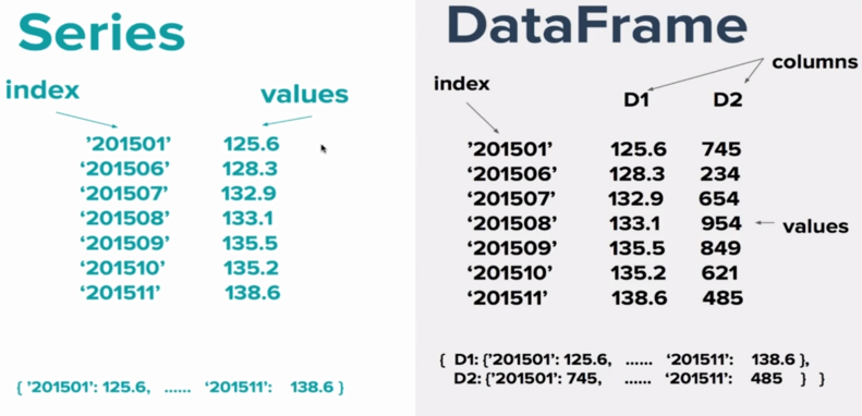
Datapandas-3 operation
Jupiter notebook creates a new file dataframe io ipynb
import numpy as np
import pandas as pd
from pandas import Series,DataFrame

import webbrowser

link = 'http://pandas.pydata.org/pandas-docs/version/0.20/io.html'
webbrowser.open(link)    # Open the browser and return True; Copy page table content
# True

df1 = pd.read_clipboard()
df1
# output
    Format Type    Data Description    Reader    Writer
0    text    CSV    read_csv    to_csv
1    text    JSON    read_json    to_json
2    text    HTML    read_html    to_html
3    text    Local clipboard    read_clipboard    to_clipboard
4    binary    MS Excel    read_excel    to_excel
5    binary    HDF5 Format    read_hdf    to_hdf
6    binary    Feather Format    read_feather    to_feather
7    binary    Msgpack    read_msgpack    to_msgpack
8    binary    Stata    read_stata    to_stata
9    binary    SAS    read_sas
10    binary    Python Pickle Format    read_pickle    to_pickle
11    SQL    SQL    read_sql    to_sql
12    SQL    Google Big Query    read_gbq    to_gbq

df1.to_clipboard()
df1
# output
    Format Type    Data Description    Reader    Writer
0    text    CSV    read_csv    to_csv
1    text    JSON    read_json    to_json
2    text    HTML    read_html    to_html
3    text    Local clipboard    read_clipboard    to_clipboard
4    binary    MS Excel    read_excel    to_excel
5    binary    HDF5 Format    read_hdf    to_hdf
6    binary    Feather Format    read_feather    to_feather
7    binary    Msgpack    read_msgpack    to_msgpack
8    binary    Stata    read_stata    to_stata
9    binary    SAS    read_sas
10    binary    Python Pickle Format    read_pickle    to_pickle
11    SQL    SQL    read_sql    to_sql
12    SQL    Google Big Query    read_gbq    to_gbq

df1.to_csv('df1.csv')
!ls   # windows system is available! dir
# DataFrame IO.ipynb    df1.csv

!more df1.csv
# output
,Format Type,Data Description,Reader,Writer
0,text,CSV,read_csv,to_csv
1,text,JSON,read_json,to_json
2,text,HTML,read_html,to_html
3,text,Local clipboard,read_clipboard,to_clipboard
4,binary,MS Excel,read_excel,to_excel
5,binary,HDF5 Format,read_hdf,to_hdf
6,binary,Feather Format,read_feather,to_feather
7,binary,Msgpack,read_msgpack,to_msgpack
8,binary,Stata,read_stata,to_stata
9,binary,SAS,read_sas,
10,binary,Python Pickle Format,read_pickle,to_pickle
11,SQL,SQL,read_sql,to_sql
12,SQL,Google Big Query,read_gbq,to_gbq

df1.to_csv('df1.csv',index=False)    # Remove index
!ls
# DataFrame IO.ipynb    df1.csv

!more df1.csv
# output
Format Type,Data Description,Reader,Writer
text,CSV,read_csv,to_csv
text,JSON,read_json,to_json
text,HTML,read_html,to_html
text,Local clipboard,read_clipboard,to_clipboard
binary,MS Excel,read_excel,to_excel
binary,HDF5 Format,read_hdf,to_hdf
binary,Feather Format,read_feather,to_feather
binary,Msgpack,read_msgpack,to_msgpack
binary,Stata,read_stata,to_stata
binary,SAS,read_sas,
binary,Python Pickle Format,read_pickle,to_pickle
SQL,SQL,read_sql,to_sql
SQL,Google Big Query,read_gbq,to_gbq

df2 = pd.read_csv('df1.csv')
df2
# output
    Format Type    Data Description    Reader    Writer
0    text    CSV    read_csv    to_csv
1    text    JSON    read_json    to_json
2    text    HTML    read_html    to_html
3    text    Local clipboard    read_clipboard    to_clipboard
4    binary    MS Excel    read_excel    to_excel
5    binary    HDF5 Format    read_hdf    to_hdf
6    binary    Feather Format    read_feather    to_feather
7    binary    Msgpack    read_msgpack    to_msgpack
8    binary    Stata    read_stata    to_stata
9    binary    SAS    read_sas
10    binary    Python Pickle Format    read_pickle    to_pickle
11    SQL    SQL    read_sql    to_sql
12    SQL    Google Big Query    read_gbq    to_gbq

df1.to_json()
# output
'{"Format Type":{"0":"text","1":"text","2":"text","3":"text","4":"binary","5":"binary","6":"binary","7":"binary","8":"binary","9":"binary","10":"binary","11":"SQL","12":"SQL"},"Data Description":{"0":"CSV","1":"JSON","2":"HTML","3":"Local clipboard","4":"MS Excel","5":"HDF5 Format","6":"Feather Format","7":"Msgpack","8":"Stata","9":"SAS","10":"Python Pickle Format","11":"SQL","12":"Google Big Query"},"Reader":{"0":"read_csv","1":"read_json","2":"read_html","3":"read_clipboard","4":"read_excel","5":"read_hdf","6":"read_feather","7":"read_msgpack","8":"read_stata","9":"read_sas","10":"read_pickle","11":"read_sql","12":"read_gbq"},"Writer":{"0":"to_csv","1":"to_json","2":"to_html","3":"to_clipboard","4":"to_excel","5":"to_hdf","6":"to_feather","7":"to_msgpack","8":"to_stata","9":" ","10":"to_pickle","11":"to_sql","12":"to_gbq"}}'

pd.read_json(df1.to_json())
# output
    Format Type    Data Description    Reader    Writer
0    text    CSV    read_csv    to_csv
1    text    JSON    read_json    to_json
2    text    HTML    read_html    to_html
3    text    Local clipboard    read_clipboard    to_clipboard
4    binary    MS Excel    read_excel    to_excel
5    binary    HDF5 Format    read_hdf    to_hdf
6    binary    Feather Format    read_feather    to_feather
7    binary    Msgpack    read_msgpack    to_msgpack
8    binary    Stata    read_stata    to_stata
9    binary    SAS    read_sas
10    binary    Python Pickle Format    read_pickle    to_pickle
11    SQL    SQL    read_sql    to_sql
12    SQL    Google Big Query    read_gbq    to_gbq


df1.to_html()
# output
'<table border="1" class="dataframe">\n  <thead>\n    <tr style="text-align: right;">\n      <th></th>\n      <th>Format Type</th>\n      <th>Data Description</th>\n      <th>Reader</th>\n      <th>Writer</th>\n    </tr>\n  </thead>\n  <tbody>\n    <tr>\n      <th>0</th>\n      <td>text</td>\n      <td>CSV</td>\n      <td>read_csv</td>\n      <td>to_csv</td>\n    </tr>\n    <tr>\n      <th>1</th>\n      <td>text</td>\n      <td>JSON</td>\n      <td>read_json</td>\n      <td>to_json</td>\n    </tr>\n    <tr>\n      <th>2</th>\n      <td>text</td>\n      <td>HTML</td>\n      <td>read_html</td>\n      <td>to_html</td>\n    </tr>\n    <tr>\n      <th>3</th>\n      <td>text</td>\n      <td>Local clipboard</td>\n      <td>read_clipboard</td>\n      <td>to_clipboard</td>\n    </tr>\n    <tr>\n      <th>4</th>\n      <td>binary</td>\n      <td>MS Excel</td>\n      <td>read_excel</td>\n      <td>to_excel</td>\n    </tr>\n    <tr>\n      <th>5</th>\n      <td>binary</td>\n      <td>HDF5 Format</td>\n      <td>read_hdf</td>\n      <td>to_hdf</td>\n    </tr>\n    <tr>\n      <th>6</th>\n      <td>binary</td>\n      <td>Feather Format</td>\n      <td>read_feather</td>\n      <td>to_feather</td>\n    </tr>\n    <tr>\n      <th>7</th>\n      <td>binary</td>\n      <td>Msgpack</td>\n      <td>read_msgpack</td>\n      <td>to_msgpack</td>\n    </tr>\n    <tr>\n      <th>8</th>\n      <td>binary</td>\n      <td>Stata</td>\n      <td>read_stata</td>\n      <td>to_stata</td>\n    </tr>\n    <tr>\n      <th>9</th>\n      <td>binary</td>\n      <td>SAS</td>\n      <td>read_sas</td>\n      <td></td>\n    </tr>\n    <tr>\n      <th>10</th>\n      <td>binary</td>\n      <td>Python Pickle Format</td>\n      <td>read_pickle</td>\n      <td>to_pickle</td>\n    </tr>\n    <tr>\n      <th>11</th>\n      <td>SQL</td>\n      <td>SQL</td>\n      <td>read_sql</td>\n      <td>to_sql</td>\n    </tr>\n    <tr>\n      <th>12</th>\n      <td>SQL</td>\n      <td>Google Big Query</td>\n      <td>read_gbq</td>\n      <td>to_gbq</td>\n    </tr>\n  </tbody>\n</table>'

df1.to_html('df1.html')
!ls
# DataFrame IO.ipynb    df1.csv        df1.html
df1.to_excel('df1.xlsx')
3-5 Selecting and indexing of dataframe
Jupiter notebook creating a new file selecting and indexing ipynb
import numpy as np
import pandas as pd
from pandas import Series, DataFrame

!pwd    # pwd corresponds to windows system chdir
# /Users/xxx/xx

!ls /Users/xxx/xx/homework    # ls corresponds to windows system dir pwd
# movie_metadata.csv

imdb = pd.read_csv('/Users/xxx/xx/homework/movie_metadata.csv')
imdb
# output
color    director_name    num_critic_for_reviews    duration    director_facebook_likes    actor_3_facebook_likes    actor_2_name    actor_1_facebook_likes    gross    genres    ...    num_user_for_reviews    language    country    content_rating    budget    title_year    actor_2_facebook_likes    imdb_score    aspect_ratio    movie_facebook_likes
0    Color    James Cameron    723.0    178.0    0.0    855.0    Joel David Moore    1000.0    760505847.0    Action|Adventure|Fantasy|Sci-Fi    ...    3054.0    English    USA    PG-13    237000000.0    2009.0    936.0    7.9    1.78    33000
1    Color    Gore Verbinski    302.0    169.0    563.0    1000.0    Orlando Bloom    40000.0    309404152.0    Action|Adventure|Fantasy    ...    1238.0    English    USA    PG-13    300000000.0    2007.0    5000.0    7.1    2.35    0
2    Color    Sam Mendes    602.0    148.0    0.0    161.0    Rory Kinnear    11000.0    200074175.0    Action|Adventure|Thriller    ...    994.0    English    UK    PG-13    245000000.0    2015.0    393.0    6.8    2.35    85000
3    Color    Christopher Nolan    813.0    164.0    22000.0    23000.0    Christian Bale    27000.0    448130642.0    Action|Thriller    ...    2701.0    English    USA    PG-13    250000000.0    2012.0    23000.0    8.5    2.35    164000
4    NaN    Doug Walker    NaN    NaN    131.0    NaN    Rob Walker    131.0    NaN    Documentary    ...    NaN    NaN    NaN    NaN    NaN    NaN    12.0    7.1    NaN    0
...    ...    ...    ...    ...    ...    ...    ...    ...    ...    ...    ...    ...    ...    ...    ...    ...    ...    ...    ...    ...    ...
5038    Color    Scott Smith    1.0    87.0    2.0    318.0    Daphne Zuniga    637.0    NaN    Comedy|Drama    ...    6.0    English    Canada    NaN    NaN    2013.0    470.0    7.7    NaN    84
5039    Color    NaN    43.0    43.0    NaN    319.0    Valorie Curry    841.0    NaN    Crime|Drama|Mystery|Thriller    ...    359.0    English    USA    TV-14    NaN    NaN    593.0    7.5    16.00    32000
5040    Color    Benjamin Roberds    13.0    76.0    0.0    0.0    Maxwell Moody    0.0    NaN    Drama|Horror|Thriller    ...    3.0    English    USA    NaN    1400.0    2013.0    0.0    6.3    NaN    16
5041    Color    Daniel Hsia    14.0    100.0    0.0    489.0    Daniel Henney    946.0    10443.0    Comedy|Drama|Romance    ...    9.0    English    USA    PG-13    NaN    2012.0    719.0    6.3    2.35    660
5042    Color    Jon Gunn    43.0    90.0    16.0    16.0    Brian Herzlinger    86.0    85222.0    Documentary    ...    84.0    English    USA    PG    1100.0    2004.0    23.0    6.6    1.85    456
5043 rows × 28 columns

imdb.shape
# (5043, 28)

imdb.head()
# output
    color    director_name    num_critic_for_reviews    duration    director_facebook_likes    actor_3_facebook_likes    actor_2_name    actor_1_facebook_likes    gross    genres    ...    num_user_for_reviews    language    country    content_rating    budget    title_year    actor_2_facebook_likes    imdb_score    aspect_ratio    movie_facebook_likes
0    Color    James Cameron    723.0    178.0    0.0    855.0    Joel David Moore    1000.0    760505847.0    Action|Adventure|Fantasy|Sci-Fi    ...    3054.0    English    USA    PG-13    237000000.0    2009.0    936.0    7.9    1.78    33000
1    Color    Gore Verbinski    302.0    169.0    563.0    1000.0    Orlando Bloom    40000.0    309404152.0    Action|Adventure|Fantasy    ...    1238.0    English    USA    PG-13    300000000.0    2007.0    5000.0    7.1    2.35    0
2    Color    Sam Mendes    602.0    148.0    0.0    161.0    Rory Kinnear    11000.0    200074175.0    Action|Adventure|Thriller    ...    994.0    English    UK    PG-13    245000000.0    2015.0    393.0    6.8    2.35    85000
3    Color    Christopher Nolan    813.0    164.0    22000.0    23000.0    Christian Bale    27000.0    448130642.0    Action|Thriller    ...    2701.0    English    USA    PG-13    250000000.0    2012.0    23000.0    8.5    2.35    164000
4    NaN    Doug Walker    NaN    NaN    131.0    NaN    Rob Walker    131.0    NaN    Documentary    ...    NaN    NaN    NaN    NaN    NaN    NaN    12.0    7.1    NaN    0
5 rows × 28 columns

imdb.tail(10)
# output
color    director_name    num_critic_for_reviews    duration    director_facebook_likes    actor_3_facebook_likes    actor_2_name    actor_1_facebook_likes    gross    genres    ...    num_user_for_reviews    language    country    content_rating    budget    title_year    actor_2_facebook_likes    imdb_score    aspect_ratio    movie_facebook_likes
5033    Color    Shane Carruth    143.0    77.0    291.0    8.0    David Sullivan    291.0    424760.0    Drama|Sci-Fi|Thriller    ...    371.0    English    USA    PG-13    7000.0    2004.0    45.0    7.0    1.85    19000
5034    Color    Neill Dela Llana    35.0    80.0    0.0    0.0    Edgar Tancangco    0.0    70071.0    Thriller    ...    35.0    English    Philippines    Not Rated    7000.0    2005.0    0.0    6.3    NaN    74
5035    Color    Robert Rodriguez    56.0    81.0    0.0    6.0    Peter Marquardt    121.0    2040920.0    Action|Crime|Drama|Romance|Thriller    ...    130.0    Spanish    USA    R    7000.0    1992.0    20.0    6.9    1.37    0
5036    Color    Anthony Vallone    NaN    84.0    2.0    2.0    John Considine    45.0    NaN    Crime|Drama    ...    1.0    English    USA    PG-13    3250.0    2005.0    44.0    7.8    NaN    4
5037    Color    Edward Burns    14.0    95.0    0.0    133.0    Caitlin FitzGerald    296.0    4584.0    Comedy|Drama    ...    14.0    English    USA    Not Rated    9000.0    2011.0    205.0    6.4    NaN    413
5038    Color    Scott Smith    1.0    87.0    2.0    318.0    Daphne Zuniga    637.0    NaN    Comedy|Drama    ...    6.0    English    Canada    NaN    NaN    2013.0    470.0    7.7    NaN    84
5039    Color    NaN    43.0    43.0    NaN    319.0    Valorie Curry    841.0    NaN    Crime|Drama|Mystery|Thriller    ...    359.0    English    USA    TV-14    NaN    NaN    593.0    7.5    16.00    32000
5040    Color    Benjamin Roberds    13.0    76.0    0.0    0.0    Maxwell Moody    0.0    NaN    Drama|Horror|Thriller    ...    3.0    English    USA    NaN    1400.0    2013.0    0.0    6.3    NaN    16
5041    Color    Daniel Hsia    14.0    100.0    0.0    489.0    Daniel Henney    946.0    10443.0    Comedy|Drama|Romance    ...    9.0    English    USA    PG-13    NaN    2012.0    719.0    6.3    2.35    660
5042    Color    Jon Gunn    43.0    90.0    16.0    16.0    Brian Herzlinger    86.0    85222.0    Documentary    ...    84.0    English    USA    PG    1100.0    2004.0    23.0    6.6    1.85    456
10 rows × 28 columns

imdb['color']
# output
0       Color
1       Color
2       Color
3       Color
4         NaN
        ...
5038    Color
5039    Color
5040    Color
5041    Color
5042    Color
Name: color, Length: 5043, dtype: object

imdb['color'][0]
# 'Color'
imdb['color'][1]
# 'Color'

imdb[['color','director_name']]
# output
    color    director_name
0    Color    James Cameron
1    Color    Gore Verbinski
2    Color    Sam Mendes
3    Color    Christopher Nolan
4    NaN    Doug Walker
...    ...    ...
5038    Color    Scott Smith
5039    Color    NaN
5040    Color    Benjamin Roberds
5041    Color    Daniel Hsia
5042    Color    Jon Gunn
5043 rows × 2 columns

sub_df = imdb[['director_name','movie_title','imdb_score']]
sub_df
# output
director_name    movie_title    imdb_score
0    James Cameron    Avatar    7.9
1    Gore Verbinski    Pirates of the Caribbean: At World's End    7.1
2    Sam Mendes    Spectre    6.8
3    Christopher Nolan    The Dark Knight Rises    8.5
4    Doug Walker    Star Wars: Episode VII - The Force Awakens  ...    7.1
...    ...    ...    ...
5038    Scott Smith    Signed Sealed Delivered    7.7
5039    NaN    The Following    7.5
5040    Benjamin Roberds    A Plague So Pleasant    6.3
5041    Daniel Hsia    Shanghai Calling    6.3
5042    Jon Gunn    My Date with Drew    6.6
5043 rows × 3 columns

sub_df.head()
# output
    director_name    movie_title    imdb_score
0    James Cameron    Avatar    7.9
1    Gore Verbinski    Pirates of the Caribbean: At World's End    7.1
2    Sam Mendes    Spectre    6.8
3    Christopher Nolan    The Dark Knight Rises    8.5
4    Doug Walker    Star Wars: Episode VII - The Force Awakens  ...    7.1

sub_df.head(5)
# output
    director_name    movie_title    imdb_score
0    James Cameron    Avatar    7.9
1    Gore Verbinski    Pirates of the Caribbean: At World's End    7.1
2    Sam Mendes    Spectre    6.8
3    Christopher Nolan    The Dark Knight Rises    8.5
4    Doug Walker    Star Wars: Episode VII - The Force Awakens  ...    7.1

sub_df.iloc[10:20,:]
# output
    director_name    movie_title    imdb_score
10    Zack Snyder    Batman v Superman: Dawn of Justice    6.9
11    Bryan Singer    Superman Returns    6.1
12    Marc Forster    Quantum of Solace    6.7
13    Gore Verbinski    Pirates of the Caribbean: Dead Man's Chest    7.3
14    Gore Verbinski    The Lone Ranger    6.5
15    Zack Snyder    Man of Steel    7.2
16    Andrew Adamson    The Chronicles of Narnia: Prince Caspian    6.6
17    Joss Whedon    The Avengers    8.1
18    Rob Marshall    Pirates of the Caribbean: On Stranger Tides    6.7
19    Barry Sonnenfeld    Men in Black 3    6.8

sub_df.iloc[10:20,0:2]
# output
director_name    movie_title
10    Zack Snyder    Batman v Superman: Dawn of Justice
11    Bryan Singer    Superman Returns
12    Marc Forster    Quantum of Solace
13    Gore Verbinski    Pirates of the Caribbean: Dead Man's Chest
14    Gore Verbinski    The Lone Ranger
15    Zack Snyder    Man of Steel
16    Andrew Adamson    The Chronicles of Narnia: Prince Caspian
17    Joss Whedon    The Avengers
18    Rob Marshall    Pirates of the Caribbean: On Stranger Tides
19    Barry Sonnenfeld    Men in Black 3

tmp_df = sub_df.iloc[10:20,0:2]
tmp_df
# output
director_name    movie_title
10    Zack Snyder    Batman v Superman: Dawn of Justice
11    Bryan Singer    Superman Returns
12    Marc Forster    Quantum of Solace
13    Gore Verbinski    Pirates of the Caribbean: Dead Man's Chest
14    Gore Verbinski    The Lone Ranger
15    Zack Snyder    Man of Steel
16    Andrew Adamson    The Chronicles of Narnia: Prince Caspian
17    Joss Whedon    The Avengers
18    Rob Marshall    Pirates of the Caribbean: On Stranger Tides
19    Barry Sonnenfeld    Men in Black 3

tmp_df.iloc[2:4,:]
# output
    director_name    movie_title
12    Marc Forster    Quantum of Solace
13    Gore Verbinski    Pirates of the Caribbean: Dead Man's Chest

tmp_df.loc[15:17,:]
# output
    director_name    movie_title
15    Zack Snyder    Man of Steel
16    Andrew Adamson    The Chronicles of Narnia: Prince Caspian
17    Joss Whedon    The Avengers

tmp_df.loc[15:17,:'movie_title']
# output
    director_name    movie_title
15    Zack Snyder    Man of Steel
16    Andrew Adamson    The Chronicles of Narnia: Prince Caspian
17    Joss Whedon    The Avengers

tmp_df.loc[15:17,:'director_name']
# output
    director_name
15    Zack Snyder
16    Andrew Adamson
17    Joss Whedon
3-6 Reindexing of series and Dataframe
Jupiter notebook creates a new file reindexing series and dataframe ipynb
import numpy as np
import pandas as pd
from pandas import Series, DataFrame

# series reindex
s1 = Series([1,2,3,4], index=['A','B','C','D'])
s1
# output
A    1
B    2
C    3
D    4
dtype: int64

# s1.reindex()    # Move the cursor over the method, press shift+tab to pop up the document, and press continuously to select the document detail level
s1.reindex(index=['A','B','C','D','E'])
# output
A    1.0
B    2.0
C    3.0
D    4.0
E    NaN
dtype: float64

s1.reindex(index=['A','B','C','D','E'],fill_value=0)
# output
A    1
B    2
C    3
D    4
E    0
dtype: int64

s1.reindex(index=['A','B','C','D','E'],fill_value=10)
# output
A     1
B     2
C     3
D     4
E    10
dtype: int64

s2 = Series(['A','B','C'], index=[1,5,10])
s2
# output
1     A
5     B
10    C
dtype: object

s2.reindex(index=range(15))
# output
0     NaN
1       A
2     NaN
3     NaN
4     NaN
5       B
6     NaN
7     NaN
8     NaN
9     NaN
10      C
11    NaN
12    NaN
13    NaN
14    NaN
dtype: object

s2.reindex(index=range(15),method='ffill')
# output
0     NaN
1       A
2       A
3       A
4       A
5       B
6       B
7       B
8       B
9       B
10      C
11      C
12      C
13      C
14      C
dtype: object

# reindex dataframe
df1 = DataFrame(np.random.rand(25).reshape([5,5]))
df1
# output
    0    1    2    3    4
0    0.255424    0.315708    0.951327    0.423676    0.975377
1    0.087594    0.192460    0.502268    0.534926    0.423024
2    0.817002    0.113410    0.468270    0.410297    0.278942
3    0.315239    0.018933    0.133764    0.240001    0.910754
4    0.267342    0.451077    0.282865    0.170235    0.898429


df1 = DataFrame(np.random.rand(25).reshape([5,5]), index=['A','B','D','E','F'], columns=['c1','c2','c3','c4','c5'])
df1
# output
    c1    c2    c3    c4    c5
A    0.278063    0.894546    0.932129    0.178442    0.303684
B    0.186239    0.260677    0.708358    0.275914    0.369878
D    0.786987    0.125907    0.191987    0.338194    0.009877
E    0.192269    0.909661    0.227301    0.343989    0.610203
F    0.503267    0.306472    0.197467    0.063800    0.813786

df1.reindex(index=['A','B','C','D','E','F'])
# output
    c1    c2    c3    c4    c5
A    0.278063    0.894546    0.932129    0.178442    0.303684
B    0.186239    0.260677    0.708358    0.275914    0.369878
C    NaN    NaN    NaN    NaN    NaN
D    0.786987    0.125907    0.191987    0.338194    0.009877
E    0.192269    0.909661    0.227301    0.343989    0.610203
F    0.503267    0.306472    0.197467    0.063800    0.813786

df1.reindex(columns=['c1','c2','c3','c4','c5','c6'])
# output
    c1    c2    c3    c4    c5    c6
A    0.278063    0.894546    0.932129    0.178442    0.303684    NaN
B    0.186239    0.260677    0.708358    0.275914    0.369878    NaN
D    0.786987    0.125907    0.191987    0.338194    0.009877    NaN
E    0.192269    0.909661    0.227301    0.343989    0.610203    NaN
F    0.503267    0.306472    0.197467    0.063800    0.813786    NaN

df1.reindex(index=['A','B','C','D','E','F'],columns=['c1','c2','c3','c4','c5','c6'])
# output
    c1    c2    c3    c4    c5    c6
A    0.278063    0.894546    0.932129    0.178442    0.303684    NaN
B    0.186239    0.260677    0.708358    0.275914    0.369878    NaN
C    NaN    NaN    NaN    NaN    NaN    NaN
D    0.786987    0.125907    0.191987    0.338194    0.009877    NaN
E    0.192269    0.909661    0.227301    0.343989    0.610203    NaN
F    0.503267    0.306472    0.197467    0.063800    0.813786    NaN


s1
# output
A    1
B    2
C    3
D    4
dtype: int64

s1.reindex(index=['A','B'])
# output
A    1
B    2
dtype: int64


df1
# output
    c1    c2    c3    c4    c5
A    0.278063    0.894546    0.932129    0.178442    0.303684
B    0.186239    0.260677    0.708358    0.275914    0.369878
D    0.786987    0.125907    0.191987    0.338194    0.009877
E    0.192269    0.909661    0.227301    0.343989    0.610203
F    0.503267    0.306472    0.197467    0.063800    0.813786

df1.reindex(index=['A','B'])
# output
    c1    c2    c3    c4    c5
A    0.278063    0.894546    0.932129    0.178442    0.303684
B    0.186239    0.260677    0.708358    0.275914    0.369878

s1
# output
A    1
B    2
C    3
D    4
dtype: int64

s1.drop('A')
# output
B    2
C    3
D    4
dtype: int64

df1
# output
    c1    c2    c3    c4    c5
A    0.278063    0.894546    0.932129    0.178442    0.303684
B    0.186239    0.260677    0.708358    0.275914    0.369878
D    0.786987    0.125907    0.191987    0.338194    0.009877
E    0.192269    0.909661    0.227301    0.343989    0.610203
F    0.503267    0.306472    0.197467    0.063800    0.813786

df1.drop('A',axis=0)
# output
    c1    c2    c3    c4    c5
B    0.186239    0.260677    0.708358    0.275914    0.369878
D    0.786987    0.125907    0.191987    0.338194    0.009877
E    0.192269    0.909661    0.227301    0.343989    0.610203
F    0.503267    0.306472    0.197467    0.063800    0.813786

df1.drop('c1',axis=0)
# An error is reported. There is no such field in the line

df1.drop('c1',axis=1)
# output
    c2    c3    c4    c5
A    0.894546    0.932129    0.178442    0.303684
B    0.260677    0.708358    0.275914    0.369878
D    0.125907    0.191987    0.338194    0.009877
E    0.909661    0.227301    0.343989    0.610203
F    0.306472    0.197467    0.063800    0.813786
3-7 talk about NaN
Jupyter notebook create a new file talk about Nan ipynb
# NaN - means Not a Number
import numpy as np
import pandas as pd
from pandas import Series, DataFrame

n = np.nan
type(n)
# float

m = 1
m + n
# nan


# Nan in Series
s1 = Series([1, 2, np.nan, 3, 4], index=['A','B','C','D','E'])
s1
# output
A    1.0
B    2.0
C    NaN
D    3.0
E    4.0
dtype: float64

s1.isnull()
# output
A    False
B    False
C     True
D    False
E    False
dtype: bool

s1.notnull()
# output
A     True
B     True
C    False
D     True
E     True
dtype: bool

s1
# output
A    1.0
B    2.0
C    NaN
D    3.0
E    4.0
dtype: float64

s1.dropna()
# output
A    1.0
B    2.0
D    3.0
E    4.0
dtype: float64

# Nan in DataFrame
dframe = DataFrame([[1,2,3],[np.nan,5,6],[7,np.nan,9],[np.nan,np.nan,np.nan]])
dframe
# output
    0    1    2
0    1.0    2.0    3.0
1    NaN    5.0    6.0
2    7.0    NaN    9.0
3    NaN    NaN    NaN

dframe.isnull()
# output
    0    1    2
0    False    False    False
1    True    False    False
2    False    True    False
3    True    True    True

dframe.notnull()
# output
    0    1    2
0    True    True    True
1    False    True    True
2    True    False    True
3    False    False    False

df1 = dframe.dropna(axis=0)
df1
# output
    0    1    2
0    1.0    2.0    3.0


df1 = dframe.dropna(axis=1)
df1
# output
0
1
2
3

df1 = dframe.dropna(axis=1,how='any')
df1
# output
0
1
2
3

# output
df1 = dframe.dropna(axis=0,how='any')
df1
# output
    0    1    2
0    1.0    2.0    3.0

df1 = dframe.dropna(axis=0,how='all')
df1
# output
    0    1    2
0    1.0    2.0    3.0
1    NaN    5.0    6.0
2    7.0    NaN    9.0

dframe2 = DataFrame([[1,2,3,np.nan],[2,np.nan,5,6],[np.nan,7,np.nan,9],[1,np.nan,np.nan,np.nan]])
dframe2
# output
    0    1    2    3
0    1.0    2.0    3.0    NaN
1    2.0    NaN    5.0    6.0
2    NaN    7.0    NaN    9.0
3    1.0    NaN    NaN    NaN

df2 = dframe2.dropna(thresh=None)
df2
# output
0    1    2    3

df2 = dframe2.dropna(thresh=2)
df2
# output
    0    1    2    3
0    1.0    2.0    3.0    NaN
1    2.0    NaN    5.0    6.0
2    NaN    7.0    NaN    9.0

dframe2
# output
    0    1    2    3
0    1.0    2.0    3.0    NaN
1    2.0    NaN    5.0    6.0
2    NaN    7.0    NaN    9.0
3    1.0    NaN    NaN    NaN

dframe2.fillna(value=1)
# output
    0    1    2    3
0    1.0    2.0    3.0    1.0
1    2.0    1.0    5.0    6.0
2    1.0    7.0    1.0    9.0
3    1.0    1.0    1.0    1.0

dframe2.fillna(value={0:0,1:1,2:2,3:3})    # Column fill
# output
    0    1    2    3
0    1.0    2.0    3.0    3.0
1    2.0    1.0    5.0    6.0
2    0.0    7.0    2.0    9.0
3    1.0    1.0    2.0    3.0

df1
# output
    0    1    2
0    1.0    2.0    3.0
1    NaN    5.0    6.0
2    7.0    NaN    9.0

df2
# output
    0    1    2    3
0    1.0    2.0    3.0    NaN
1    2.0    NaN    5.0    6.0
2    NaN    7.0    NaN    9.0

df1.dropna()
# output
    0    1    2
0    1.0    2.0    3.0

df1.fillna(1)
# output
    0    1    2
0    1.0    2.0    3.0
1    1.0    5.0    6.0
2    7.0    1.0    9.0