Python wechat ordering applet course video

https://edu.csdn.net/course/detail/36074

Python actual combat quantitative transaction financial management system

https://edu.csdn.net/course/detail/35475
How to input the adjacency matrix stored on disk into R program is the starting point of social network analysis. The basic data structure and code structure have been introduced in the previous chapters. This chapter will face a substantive problem, learning how to import a graph and calculate some attributes of the graph.

• File representation of a graph
• Import a graph
• Generate artificial network
• Basic analysis of graph

File representation of a graph

In computer, the basic structures of the two most common representations are adjacency matrix and adjacency table. Take the simplest undirected graph without authority as an example, the element aija in the second row and jj column of the adjacency matrix_ If {ij} is equal to 1, it means that there is an edge between vertex ii and vertex jj, that is, the adjacency matrix represents the relationship between all nodes. The adjacency table is to establish a single linked list for vertex ii. This single linked list is composed of all neighbor nodes of vertex ii, that is, the adjacency table only represents the related nodes.

Many public data sets on the network often use triples to represent a graph. The following is an example of a triple. Take the triple (1, 2, 1) in the first row as an example, which indicates that there is an edge from vertex 1 to vertex 2, and the weight of the edge is 1. For non weighted graphs, the third element in the triplet is usually omitted.

1	2	1
1	3	-1
2	3	-1
1	4	-1
3	4	1

💡 Hint

Most public datasets can be found on the following websites:

1. Stanford Large Network Dataset Collection: http://snap.stanford.edu/data

2. The KONECT Project: http://konect.cc/networks

Import a graph

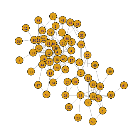
Below with Dolphins Take the network as an example and import it into the R program. Dolphin is a real network without authority and direction. It describes the bottlenose dolphin community living near a fjord in New Zealand, in which nodes represent Dolphins and edges represent the social relations between Dolphins. After downloading the dataset, open the file named out.

% sym unweighted
9	4
10	6
10	7
11	1
......

Before reading the file, you need to modify it. You can see that the first line "% sym unweighted" of the file is three elements separated by spaces. The R language is not too intelligent. When reading the second line, you will report an error because there are only two elements, so you need to delete the first line. Next, use read Table() reads the file into the R program:

graph.edges <- read.table(file = "out.dolphins", header = FALSE)

💡 Hint

You can also replace the tab (\ t) in the out file with a comma (,), change the file to a comma separated CSV file, and use read Csv() function reads.

You may be curious about the graph you read What exactly is edges? Use the class() function to see the type of variable:

> class(graph.edges)
[1] "data.frame"

data.frame doesn't seem to be introduced in the previous chapter. Limited by the research direction, this may be the only time you touch the data frame type. Don't worry about it. The read data is converted into a diagram below:

> library(igraph)
> graph <- graph_from_data_frame(graph.edges, directed = FALSE)

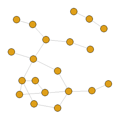
The following figure shows the imported dolphin network:

> class(graph)
[1] "igraph"
> plot(graph)

Output the scale of dolphin network:

> cat(sprintf("Nodes: %s\nEdges: %s\n", length(V(graph)), length(E(graph))))
Nodes: 62
Edges: 159

Two new functions V() and E() are used here, where V() is the point set of the graph and E() is the edge set of the graph. Most of the future analysis is based on these two sets. These two functions will accompany your R language journey until the end.

The imported network can be saved as an R file, which can be directly loaded and used next time. The experimental data can also be persisted by using the same method.

> save(graph, file = "dolphins.RData")  # Save graph variable
> load(file = "dolphins.RData")  # Import variables stored in RData files

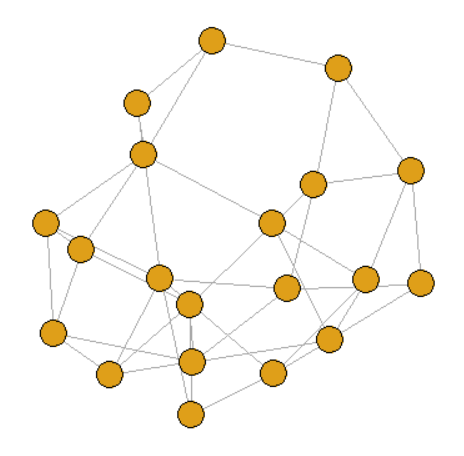
Generate artificial network

Using artificial network to verify the effectiveness of the algorithm is also an essential part of the experiment. Several common artificial network structures are introduced below.

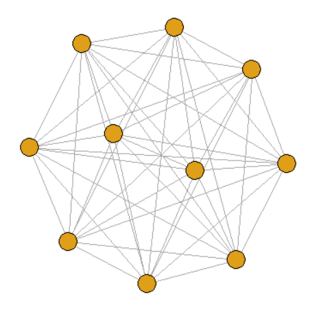
1. Full connection diagram

graph <- make_full_graph(10)

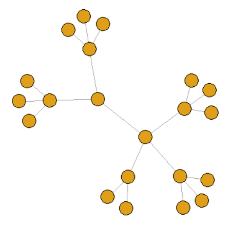
2. Tree view

graph <- make_tree(21, children = 3, mode = "undirected")

3. k-regular graph

graph <- sample_k_regular(20, 3)

4. Erdos-Renyi Random

graph <- sample_gnp(20, 0.1)

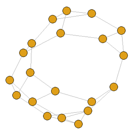
5. Small world network

graph <- sample_smallworld(dim = 1, size = 20, nei = 2, p = 0.1)

💡 Hint

For other manual structures, please check the iGraph document: https://igraph.org/r/doc

Basic analysis of graph

The above obtains the igraph graph object from the perspectives of importing external network and generating artificial network. Next, we will use the functions in the igraph package to make a simple analysis of dolphin network.

1. Judging the connectivity of Graphs

> is.connected(graph)
[1] TRUE

1. Calculate the degree of the graph

> degree(graph)  # Calculate the degree of all nodes in the graph, including the name of the first behavior node and the degree of the second behavior node
9 10 11  ...
6  7  5  ...
> degree(graph, v = "9")  # Calculate the degree of some nodes in the graph
9 
6

1. Calculate the density of the graph

> edge_density(graph)
[1] 0.0840825

1. Path analysis of graph

> diameter(graph, directed = FALSE, weights = NA)  # diameter
[1] 8
> radius(graph)  # radius
[1] 5
> distances(graph, v = V(graph)$name[1], to = V(graph)$name[10], algorithm = "unweighted", weights = NA)  # Calculate the shortest distance between nodes
  20
9  3
> shortest_paths(graph, from = "1", to = "6", weights = NA)  # Calculate the shortest path from node 1 to node 6
$vpath
$vpath[[1]]
+ 6/62 vertices, named, from e1ce364:
[1] 1  41 37 40 58 6

1. Calculate the clustering coefficient of the graph

> transitivity(graph, type = "average")
[1] 0.3029323

✏️ Practice

1. Try to download other networks from the dataset website and import them into the R program;

2. Try to calculate the average degree of import network;

3. Find the igraph document and try to calculate the assortability of the imported network.