1, Basic operation

Chinese document of pythonPytorch

https://pytorch-cn.readthedocs.io/zh/latest/package_references/torch-optim/

1, Anaconda basic operation

1,use conda establish Python Virtual environment (in) conda prompt (completed in environment)
conda create -n environment_name python=X.X

2,Activate virtual environment (in) conda prompt (completed in environment)
activate your_env_name(Virtual environment name)

3,Installing external packages for virtual environments
conda install -n your_env_name [package]

4,View existing environment(The currently active environment displays an asterisk)
conda info -e

5,Delete an existing virtual environment
conda remove --name your_env_name --all

6,Enter virtual environment
conda activate your_env_name(Virtual environment name)

2, Tensor and Numpy

tensor can easily perform convolution, activation, up and down sampling, differential derivation and other operations, while numpy array cannot

3, Back propagation method

https://blog.csdn.net/shijing_0214/article/details/51923547?utm_medium=distribute.pc_relevant.none-task-blog-BlogCommendFromMachineLearnPai2-4.control&depth_1-utm_source=distribute.pc_relevant.none-task-blog-BlogCommendFromMachineLearnPai2-4.control

4, Pytoch feature automatic gradient module Autograd

1. Core data structure Variable

variable encapsulates three data:

Data (save the tensor contained in the variable),

Grad (save the gradient corresponding to data. Grad is also a variable rather than a tensor, which is consistent with the shape of data). During the creation of variable variable, you can use requires_ The value of grad, which is used by the program to choose whether to track the value during the calculation

​ grad_ FN (point to a function to record the operation history of the tensor, that is, the output of what operation the tensor is, which is used to build the calculation diagram. If a tensor is obtained by a+b, the value of grad_fn is AddBackward. If a Variable variable is created by the user, that is, it is the leaf node, and the corresponding grad_fn is None)

If a Variable variable a -- a = V(t.ones(3, 4), requires_grad =True)

Call a.sum() and a.data The result of sum () is different. The result of the former is still Variable after calculating sum, and the result of the latter is tensor after taking data

2. Calculation diagram

5, Neural network toolbox nn

####  Tip: self in Python

1. Self must only exist in the functions of the class. Ordinary functions do not need to have self, and there is no need to assign a value to the self parameter when calling. Self represents the instance object of the class (note that it is not the class itself). Self can be replaced by other names, but the Convention is better self
2. Principle of self
   Create a class Test(), instantiate the class t=Test(), get the object T, call the method t.fun(x,y) of the object, and python will automatically turn to test fun(t,x,y)

1.nn.Module

As an automatic differential system, autograd is too low-level for the actual deep learning project. In practical use, we can use the nn toolbox module. torch. The core data structure of nn is module. In use, the most common is to inherit nn Module to write its own network layer.

1) Full connection layer Linear

The following is an example of using an existing model from the nn toolbox

in_features refers to the size of the input two-dimensional tensor, that is, the size in the input [batch_size, size].
out_features refers to the size of the output two-dimensional tensor, that is, the shape of the output two-dimensional tensor is [batch_size, output_size]. Of course, it also represents the number of neurons in the full connection layer.

[the external chain image transfer fails. The source station may have an anti-theft chain mechanism. It is recommended to save the image and upload it directly (img-e2ox8dfp-1620980777610) (C: \ users \ 15729 \ appdata \ roaming \ typora user images \ image-20210313145041022. PNG)]

The following is an example of using NN Module implements its own full connection layer (full connection layer, that is, the output y and input x meet y=wx+b, and w and b are learnable parameters)

import torch as t
from torch import nn
from torch.autograd import Variable


class Linear(nn.Module):  # Inherit NN Module
    def __init__(self, in_features, out_features):
        super(Linear, self).__init__()  # Equivalent to NN Module.__ init__ (self)
        self.w = nn.Parameter(t.randn(in_features, out_features))
        self.b = nn.Parameter(t.randn(out_features))

    def forward(self, x):
        x = x.mm(self.w)
        return x + self.b.expand_as(x)


layer = Linear(4, 3)
input = Variable(t.randn(2, 4))
output = layer(input)  #Equivalent to layer forward(input)
print(input)
print(output)

be careful

• Custom layer Linear must inherit NN Module, and NN needs to be called in its constructor Constructor of module
• In the constructor init, you must define the learnable parameters and encapsulate them into parameters. In this case, we encapsulate w and b into parameters. Parameter is a special Variable, but it requires derivation by default (requires_grad=True)
• The forward function implements a forward propagation process. Its input can be one or more variables. Any operation on x must also be supported by variables
• There is no need to write back propagation Function, because its forward propagation is to operate on variable, NN Module can automatically realize back propagation by using autograd, which is much simpler than Function
• When in use, layer can be intuitively regarded as a function in mathematical concept, and the corresponding result of input can be obtained by calling layer(input). It is equivalent to layers__ call__ (input). In the call function, the main call is layer forward(x). In practical use, layer(x) should be used instead of layer forward(x)

2) Multilayer perceptron

Activation function

In short, the activation function introduces nonlinearity to solve the classification problem that cannot be solved by linear function and single-layer perceptron

If the activation function is not used, in this case, the output of each layer is a linear function of the input of the upper layer. It is easy to verify that no matter how many layers the neural network has, the output is a linear combination of inputs, which is equivalent to the effect of no hidden layer. This is the most primitive Perceptron. Therefore, the nonlinear function is introduced as the activation function, so the deep neural network is meaningful (it is no longer a linear combination of inputs, but can approximate any function). The earliest idea is sigmoid function or tanh function. The output is bounded and it is easy to act as the input of the next layer.

https://blog.csdn.net/qq_30815237/article/details/86700680

In the case of the above Linear, we can add multi layers to realize multi-layer perceptron. The code is as follows:

class Perceptron(nn.Module):
    def __init__(self, in_features, hidden_features, out_features):
        nn.Module.__init__(self)
        self.layer1 = Linear(in_features, hidden_features)
        self.layer2 = Linear(hidden_features, out_features)

    def forward(self, x):
        x = self.layer1(x)
        x = t.sigmoid(x)
        return self.layer2(x)


perceptron = Perceptron(3, 4, 1)
for name, param in perceptron.named_parameters():
    print(name, param.size())

be careful

• In the constructor init, the previously customized Linear layer (module) can be used as a sub module of the current module object, and its learnable parameters will also become the learnable parameters of the current module
• In the forward propagation function, we consciously name the output variables as x, so that python can reclaim some middle-level output and save memory

The global naming specification of parameter in module is as follows:

• Parameter is named directly. For example, self param_name=nn. Parameter (t.randn (3,4)), named param_name
• The parameter in the sub module will be preceded by the name of the current module. For example, self sub_ Module = submodel(), there is a parameter in the submodel, which is also called parameter_ Name, then the parameter name formed by the combination of the two is sub_module.param_name

2. Common neural network layer

3. Optimizer

PyTorch encapsulates all the optimization methods commonly used in deep learning in torch In optim

All optimization methods inherit the base class optim Optimizer, and implemented its own optimization steps. The following is an example of the most basic optimization method - random gradient descent method (SGD). Here we need to focus on:

• Basic usage of optimization method
• How to set different learning rates for different parts of the model
• How to adjust the learning rate

Use of optimizer

To use torch Optim, you need to build an optimizer object. This object can maintain the current parameter state and update the parameters based on the calculated gradient.

structure

To build an optimizer, you need to give it an iterable containing the parameters to be optimized (which must all be Variable objects). Then, you can set the parameter options of optimizer, such as learning rate, weight attenuation, and so on

Optimization methods: https://blog.csdn.net/q295684174/article/details/79130666

//Different optimization methods and optimization rules are selected, including SGD, Adam, etc
optimizer = optim.SGD(model.parameters(), lr = 0.01, momentum=0.9)
optimizer = optim.Adam([var1, var2], lr = 0.0001) 

Set options individually for each parameter

If you want to do this, do not directly pass in the iterable of Variable, but the iterable of dict. Each dict defines a set of parameters and contains a param key, which corresponds to the list of parameters. Other keys should match the keywords of other parameters accepted by optimizer and will be used to optimize this set of parameters.

For example, this is useful when we want to specify the learning rate of each layer:

optim.SGD([
                {'params': model.base.parameters()},
                {'params': model.classifier.parameters(), 'lr': 1e-3}
            ], lr=1e-2, momentum=0.9)

This means model The parameters of base will use the learning rate of 1e-2, model Classifier parameters will use 1e-3 learning rate, and 0.9 momentum will be used for all parameters.

Execution optimization

All optimizer s implement the step() method, which updates all parameters. It can be used in two ways:

optimizer.step()

This is a simplified version supported by most optimizer s. Once the gradient is calculated by a function such as backward(), we can call this function.

optimizer.step(closure)

Some optimization algorithms, such as converge gradient and LBFGS, need to calculate functions repeatedly, so you need to pass in a closure to allow them to recalculate your model. This closure should empty the gradient, calculate the loss, and then return.

Adjust learning rate

There are two main ways to adjust the learning rate. One is to modify optimizer param_ The other is to create a new optimizer (which is simpler and more recommended). Because the optimizer is very lightweight and the construction cost is very small, a new optimizer can be built. However, the new optimizer will reinitialize the momentum and other state information, which may cause the loss function to oscillate in the convergence process for the optimizer using momentum (such as SGD with momentum)

# Adjust the learning rate and create an optimizer
old_lr=0.1

optimizer=optim.SGD([
    {'params':net.features.parameters()},
    {'params':net.classifier.parameters(),'lr':old_lr*0.1}
],lr=1e-5)

4.nn.functional

Most layer s in nn have a corresponding function in functional.

​ nn.functional and NN The main differences between modules are:

layers implemented with Moudule is a special class, which will automatically extract the parameters of the science department

Functions in functional are more like pure functions, defined by def function(input)

When the model has learnable parameters, it is best to use NN Module, otherwise you can use NN functional

5. Save data

remove none
torch.save(net1 ,'net.pth')

Parameter retention
torch.save(net1.state_dict(), 'net_params.pth' )

Load the saved model

net = Net()

net.load_state_dict(t.load('net.pth'))

6, Tools commonly used in pytoch

1. Data processing

(1) Data loading, Dataset

In pytorch, data loading can be realized through custom dataset objects. The dataset object is abstracted as a dataset class. When we use this class to process our own dataset, we must inherit the dataset class (in the torch.utils.data package, it is called through data.Dataset) and implement its two magic methods.

1. __ getitem__(index):

   Return a sample data. When obj[index] is used, it is actually calling obj__ getitem__ (index)

2. __ len__():

   Returns the number of samples. When len(obj) is used, obj is actually called__ len__ ()

For example:

class dogCat(data.Dataset):
    def __init__(self,root): # root is the data storage directory
        imgs = os.listdir(root) #List all files in the current path
        self.imgs = [os.path.join(root,img) for img in imgs] # Path of all pictures
        #print(self.imgs)

	"""Return a sample data"""
    def __getitem__(self, item): 
        img_path = self.imgs[item] # The path of the item picture
        #dog 1 cat 0
        label = 1 if 'dog' in img_path.split('\\')[-1] else 0 # Get tag information
        #print(label)
        pil_img = Image.open(img_path) #Read in picture
        print(type(pil_img))
        array = np.asarray(pil_img) # To numpy Array type
        data = t.from_numpy(array) # Change to tensor type
        return data,label #Return the tensor and its label corresponding to the picture

	"""Number of samples"""
    def __len__(self):
        return len(self.imgs)

(2)dataloader

Although we can record the data after encapsulating the Dataset class, we still need more steps in the actual training process:

1. Load batch size data at one time.
2. Disrupt the order of data.
3. Multithreading loads data.

All these requirements have been implemented by the DataLoader class

https://www.cnblogs.com/ranjiewen/articles/10128046.html

The operation sequence of loading pytorch data into the model is as follows:

① Create a Dataset object
② Create a DataLoader object
③ Loop the DataLoader object and load img and label into the model for training

The purpose of the DataLoader interface is to encapsulate the customized Dataset into a Tensor of batch size according to batch size and whether it is shuffle d for later training.

The following are the parameters of DataLoader(object):

• dataset(Dataset): incoming dataset
• batch_size(int, optional): how many samples are there in each batch
• shuffle(bool, optional): whether to reorder the data at the beginning of each epoch
• num_workers (int, optional): this parameter determines how many processes handle data loading. 0 means that all data will be loaded into the main process. (default = 0)

(3) Computer vision Toolkit: torch vision

For image data, the above data is not perfect when loading, because only the pictures are read in without relevant processing, such as the size and shape of each picture, the numerical normalization of samples and so on.
  in order to solve this problem, PyTorch has developed a visual toolkit torchvision, which is independent of torch and needs to be installed separately through pip install torchvision.

torchvision consists of three parts:

• Models: provide various classic network structures and pre trained models, such as AlexNet, VGG, ResNet, Inception, etc.

from torchvision import models
from torch import nn
resnet34 = models.resnet34(pretrained=True,num_classes=1000) # Load pre training model
resnet34.fc=nn.Linear(512,10) # Modify the full connection layer to 10 classification

• Datasets: provides commonly used datasets, such as MNIST, CIFAR10/100, ImageNet, COCO, etc.

from torchvision import datasets
dataset = datasets.MNIST('data/',download=True,train=False,transform=transform)

• transforms: provides common data preprocessing operations, mainly for Tensor and PIL Image objects.

Operations on PIL Image:

Scale: adjust the picture size and keep the aspect ratio unchanged

CenterCrop, RandomCrop, RandomsizedCrop: crop pictures

Pad: fill picture

ToTensor: converting PIL Image into Tensor will automatically normalize [0255] to [0,1]

Operations on Tensor: Normalize, ToPILImage, etc.

Normalize: normalize, that is, subtract the mean value and divide it by the standard deviation

ToPILImage: convert Tensor to PIL Image object

import os
from torch.utils import data
from PIL import Image
import numpy as np
from torchvision import transforms as T

transform = T.Compose([T.Resize(224),T.CenterCrop(224),T.ToTensor(),T.Normalize(mean=[.5,.5,.5],std=[.5,.5,.5])])  # Build conversion operation

class dogCat(data.Dataset):
    def __init__(self,root,transforms):
        imgs = os.listdir(root)
        #print(imgs)
        self.imgs = [os.path.join(root,img) for img in imgs]
        #print(self.imgs)
        self.transforms = transforms

    def __getitem__(self, item):
        img_path = self.imgs[item]
        #dog 1 cat 0
        label = 1 if 'dog' in img_path.split('\\')[-1] else 0
        #print(label)
        pil_img = Image.open(img_path)
        if self.transforms:
            pil_img = self.transforms(pil_img)  #Perform quasi replacement operation
        return pil_img,label,item

    def __len__(self):
        return len(self.imgs)

7, Actual development

In the research of deep learning, the program generally needs to realize the following aspects:

① model definition

② data processing and loading

③ training model

④ visualization of training process

⑤ test

The most common neural network training can be summarized as the following three steps:

① input the training data into the model and start forward propagation.
② calculate the gap between the model output and the standard answer through the loss function to obtain the loss value.
③ according to the loss value back propagation, use the optimizer to update the model parameters.

The specific training steps of pytorch are very simple:

① the data input model is output.
② calculate loss according to the output and label.
​ ③ optimizer.zero_grad() optimizer zeroes the gradient.
​ ④ loss. Backward() loss backpropagation.
​ ⑤ optimizer. The step () optimizer updates the parameters.

According to the above steps, we have completed the following training and verification modules:

def train(model, loss_fn, optimizer, dataloader, num_epochs = 1):
    for epoch in range(num_epochs):
        print('Starting epoch %d / %d' % (epoch + 1, num_epochs))

        # Validate model effect on validation set
        check_accuracy(fixed_model, image_dataloader_val)
        
        model.train() # Model The train() method allows the model to enter the training mode, the gradient of parameters is retained, and the dropout layer works normally.
        for t, sample in enumerate(dataloader):
            x_var = Variable(sample['image'])   # Get the image data of a batch.
            y_var = Variable(sample['Label'].long()) # Get the corresponding label.

            scores = model(x_var)   # Get the output.
            
            loss = loss_fn(scores, y_var)   # Calculate loss.
            if (t + 1) % print_every == 0:  # Print loss at regular intervals.
                print('t = %d, loss = %.4f' % (t + 1, loss.item()))

            # Three steps to update parameters.
            optimizer.zero_grad()
            loss.backward()
            optimizer.step()
def check_accuracy(model, loader):

    num_correct = 0
    num_samples = 0

    model.eval() # Model The eval() method switches to the evaluation mode, and the corresponding dropout and other parts will stop working.
    for t, sample in enumerate(loader):
        x_var = Variable(sample['image'])
        y_var = sample['Label']
       
        scores = model(x_var)
        _, preds = scores.data.max(1) # Find the highest possible label as output.

        num_correct += (preds.numpy() == y_var.numpy()).sum()
        num_samples += preds.size(0)
    acc = float(num_correct) / num_samples
    print('Got %d / %d correct (%.2f)' % (num_correct, num_samples, 100 * acc))

2, Basic composition of neural network

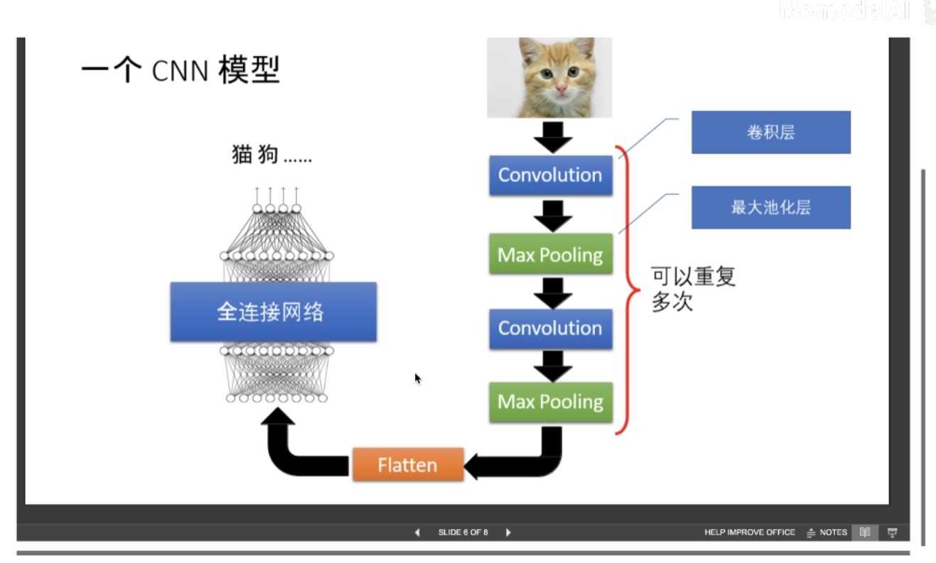
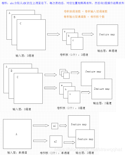
Convolution layer

Number of convolution kernel channels of CNN = number of channels of convolution input layer
Number of convolution output layer channels of CNN (depth) = number of convolution kernels (any number)

The calculation formula of output dimension of accumulation layer and pool layer is N=(W-F+2P)/S+1,

Where F is the volume kernel size, P is the padding size around the image, and S is the step size

For example: an 8 × 8 original picture, after 3 × 3 convolution kernel default convolution operation, get 6 × Picture of 6

conv2d parameters are as follows:

torch.nn.Conv2d(in_channels, out_channels, kernel_size, 
	stride=1, padding=0, dilation=1, groups=1, bias=True, padding_mode='zeros')

Assuming that the number of convolution cores of X and C is the same as the number of convolution cores of the input channel of C, it is necessary to calculate the convolution core of X (that is, the number of convolution cores of C is the number of convolution cores of C), so the convolution core of X corresponds to the input channel of C, When such a convolution kernel is applied to the input, a channel of the output is obtained. Suppose there are P convolution kernels of K x K x C, so each convolution kernel applied to the input will get a channel, so the output has P channels.

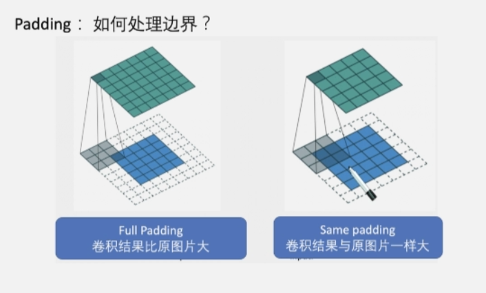
Padding

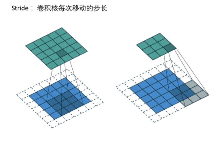
Stride

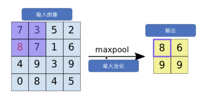
Max pool layer maxpool

The following is PyTorch's implementation of the pooling layer.

>>> import torch 
>>> from torch import nn 
# Pooling mainly requires two parameters. The first parameter represents the size of the pooling area and the second parameter represents the step size 
>>> max_pooling = nn.MaxPool2d(2, stride=2) 
>>> aver_pooling = nn.AvgPool2d(2, stride=2) 
>>> input = torch.randn(1,1,4,4) 
>>> input tensor(
    [[[[ 1.4873, -0.2228, -0.3972, -0.1336], 
       [ 0.6129, 0.4522, -0.3175, -1.2225], 
       [-1.0811, 2.3458, -0.4562, -1.9391], 
       [-0.3609, -2.0500, -1.2374, -0.2012]]]]) 
# Call the maximum value pooling and average value pooling. You can see that the size changes from [1, 1, 4, 4] to [1, 1, 2, 2] 
>>> max_pooling(input) 
	tensor([[[[ 1.4873, -0.1336], 
       		  [ 2.3458, -0.2012]]]]) 
>>> aver_pooling(input) 
	tensor([[[[ 0.5824, -0.5177],
              [-0.2866, -0.9585]]]])

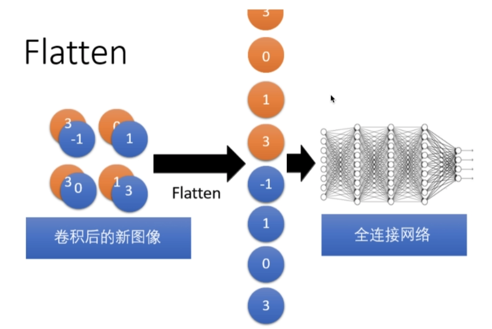
Flatten layer

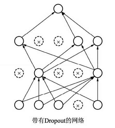
Dropout layer

In deep learning, when there are too many parameters and relatively few training samples, the model is prone to over fitting. The specific performance of over fitting is that the prediction accuracy is high in the training set, while the accuracy decreases significantly in the test set.

The basic idea of Dropout is shown in the figure. During training, each neuron is retained with probability p, that is, it stops working with probability of 1-p. the neurons retained in each forward propagation are different, which makes the model less dependent on some local features and has stronger generalization performance. During the test, in order to ensure the same expected output value, each parameter should be multiplied by P. Of course, there is another calculation method called Inverted Dropout, which multiplies the reserved neurons by 1/p during training, so there is no need to change the weight during testing.

An example of using Dropout in PyTorch is as follows:

 >>> import torch >>> from torch 
     import nn
    # PyTorch sets the element to 0 to implement the Dropout layer. The first parameter is the probability of setting 0, and the second parameter is whether to operate in place 
 >>> dropout = nn.Dropout(0.5, inplace=False) 
 >>> input = torch.randn(2, 64, 7, 7) 
 >>> output = dropout(input)

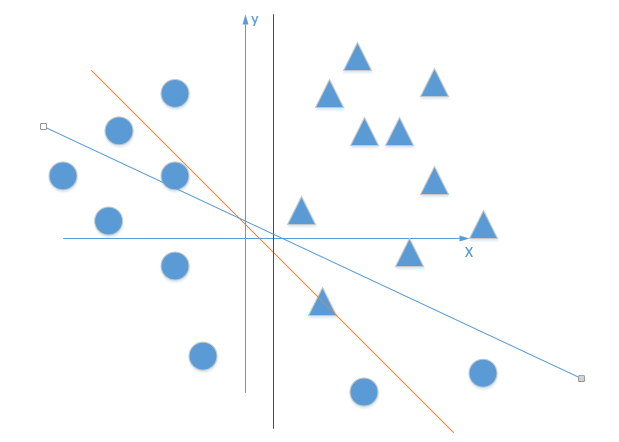
Role of full connection layer

https://www.zhihu.com/question/41037974

The main function of the full connection layer is to realize Classification

From the figure below, we can see that

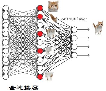
Red neurons indicate that this feature has been found (activated)

Other neurons in the same layer are either not obvious in cats or not found

When we put these features together, we found that the cat was the most qualified

PyTorch uses the full connection layer and needs to specify the dimensions of input and output. Examples are as follows:

 >>> import torch 
 >>> from torch import nn 
# The first dimension represents a total of four samples 
 >>> input = torch.randn(4, 1024) 
 >>> linear = nn.Linear(1024, 4096)
 >>> output = linear(input)
 >>> input.shape 
    torch.Size([4, 1024])
 >>> output.shape 
    torch.Size([4, 4096])

tip: robustness

The robustness of computer software is whether it does not crash and crash in the case of input error, disk failure, network overload or intentional attack.

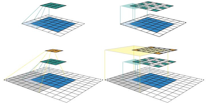
Receptive field

Receptive field is the size of the area mapped by the pixels on the * * Feature Map * * of each layer in the convolutional neural network in the original image, which is equivalent to how large the pixels in the high-level Feature Map are affected by the original image.

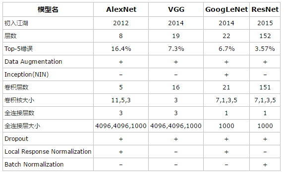
Various classical network models

During the evolution of CNN network structure, many excellent CNN networks have appeared, such as LeNet, AlexNet, VGg net, GoogLeNet, RESNET and desnet

https://blog.csdn.net/u013989576/article/details/71600795

3, Object detection framework

https://blog.csdn.net/fu_shuwu/article/details/84195998

1. Two order classical detector: fast RCNN

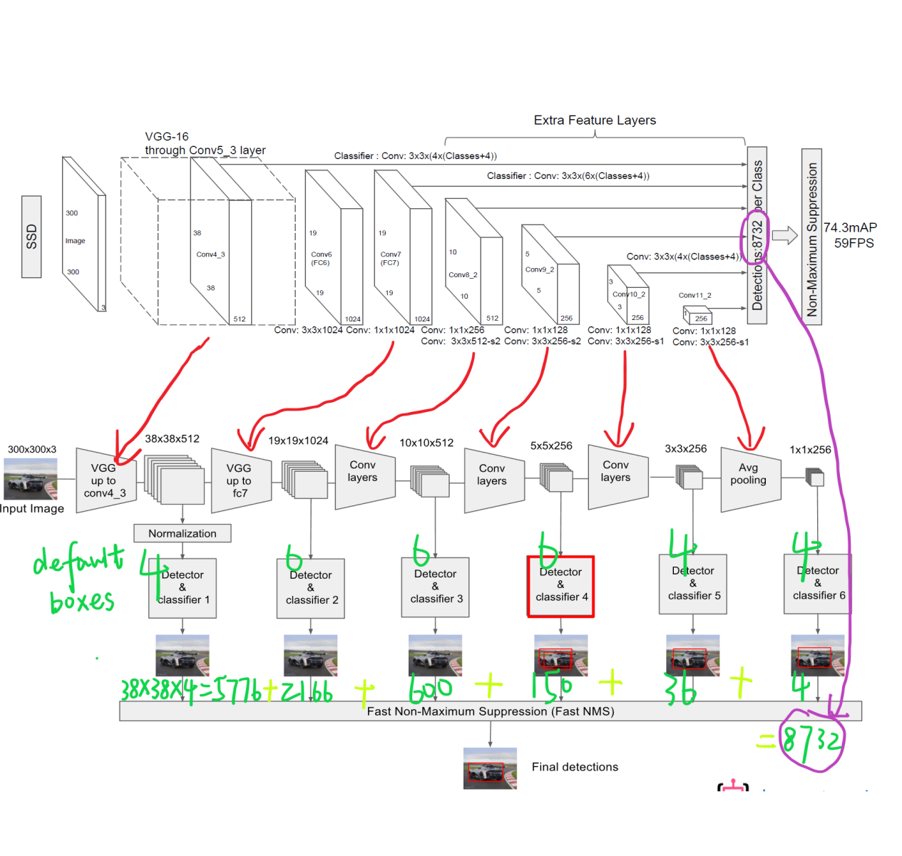
2. Single order multilayer detector: SSD

https://blog.csdn.net/weixin_40479663/article/details/82953959