Introduction notes to pytorch

Posted by iskawt on Fri, 14 Jan 2022 10:30:50 +0100

This article is my recent self-study pytorch notes, according to Introduction to pytorch Basics Please correct any mistakes or misunderstandings in the notes of what you have learned. The feelings and experiences of this teaching video are at the end of the article. Love the official account if you like. Some of your learning experience and recommendations will be shared on the official account. The official account number is at the end of the article. I hope we can go forward in 2022!

CUDA NVIDIA for hardware acceleration
Core of deep learning: gradient descent algorithm

X '(next value) = x-rate (step) * x' (reciprocal of x)

The derived gradient drops are Adam, sgd, rmsprop, nag, adadelta, adagrad and momentum

Approximate solution of Closed Form Solution

Logistic Regression compression function, compressed to 0-1

Linear Regression

Differences between Python and python data types

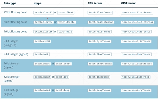
a=torch.randn(2,3)

print(a.type())#You can view specific data types
#The output is' torch FloatTensor'
print(type(a))#View basic data types, not commonly used
#torch.Tensor
print(isinstance(a,torch.FloatTensor))#Matching data type
#The output is True

#The same Tensor deployed on GPU and CPU is different
``
### Dimension0/rank0 (scalar)
torch.tensor(1.)
#Output is tensor (1.)
torch.tensor(1.3)
#Output tensor (1.300)

#Can be used to express loss

In pytoch, vectors are collectively referred to as tensors,

Dim0, scalar

Dim1: Bias Linear Input

Dim2:Linear Input batch

Dim3:RNN input Batch

Dim4:CNN:[b,c,h,w]

tensor: input ready-made data

FloatTensor input dimension (not commonly used)

list is not recommended
Path import of dataset

import os
from torch.utils.data import Dataset
from PIL import Image

class MyData(Dataset):
    def __init__(self, root_dir, label_dir):
        self.root_dir = root_dir
        self.label_dir = label_dir
        self.path = os.path.join(self.root_dir, self.label_dir)
        self.img_path = os.listdir(self.path)

    def __getitem__(self, idx):
        img_name = self.img_path[idx]
        img_item_path = os.path.join(self.root_dir, img_name)
        img = Image.open(img_item_path)
        label = self.label_dir
        return img, label

    def __len__(self):  # length
        return len(self.img_path)


root_dir = "dataset/train"
ants_label_dir = "ants"
bees_label_dir = "bees"
ants_dataset = MyData(root_dir, ants_label_dir)
bees_dataset = MyData(root_dir, bees_label_dir)

train_dataset = ants_dataset + bees_dataset  # Data set splicing. Sometimes the data is not enough, multiple similar data sets can be spliced

Use of TensorBoard (one data)

The tensor data type is required to display, so format conversion is required before use

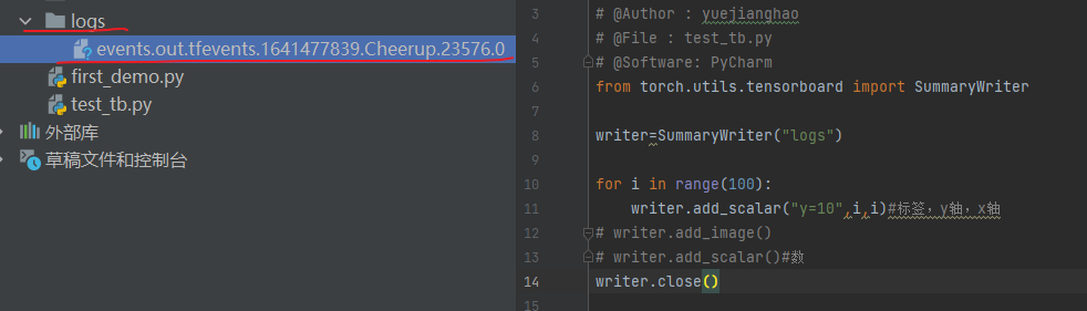
from torch.utils.tensorboard import SummaryWriter

writer=SummaryWriter("logs")

for i in range(100):
    writer.add_scalar("y=x",i,i)#Label, y-axis, x-axis
# writer.add_image()
# writer.add_scalar()#number
writer.close()

Opening method:

Enter at the terminal:

tensorboard --logdir=logs

When multiple people use it, the port may be occupied. Modify the port as follows

tensorboard --logdir=logs --port=6007

from torch.utils.tensorboard import SummaryWriter
import numpy as np
from PIL import Image

writer = SummaryWriter("logs")
image_path = "dataset/train/ants/0013035.jpg"
img_PIL = Image.open(image_path)
img_array = np.array(img_PIL)  # Convert to np type to match writer add_ Input parameters for image()
print(type(img_array))
print(img_array.shape)#It is known from (512, 768, 3) that the channel is behind, so other functions are required to convert it


writer.add_image("test",img_array,1,dataformats='HWC')#Display the picture and convert the format. Convert the format to HWC and put the channel behind. In this way, you can see the output results of each step
for i in range(100):
    writer.add_scalar("y=10", i, i)  # Label, y-axis, x-axis
writer.close()

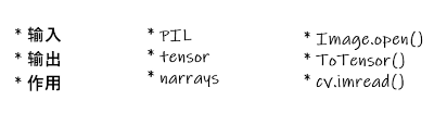
Transform to transform the picture

import cv2
from PIL import Image
from torch.utils.tensorboard import SummaryWriter
from torchvision import transforms

# Usage of python - data type of tensor
# Through transform To tensor, look at two questions
# 1. How to use transform (Python)
# 2. Why do I need Tensor data types
# Relative path is required because it is a diagonal bar and absolute path is a backslash
img_path = "dataset/train/ants/0013035.jpg"
img = Image.open(img_path)

writer=SummaryWriter("logs")

# 1. How to use transform (Python)
tensor_trans = transforms.ToTensor()
tensor_img = tensor_trans(img)

#Introducing pictures using cv2
cv_img=cv2.imread(img_path)

writer.add_image("Tensor_img",tensor_img)
writer.close()

from PIL import Image
from torch.utils.tensorboard import SummaryWriter
from torchvision import transforms

writer = SummaryWriter("logs")
img = Image.open("dataset/train/ants/0013035.jpg")
print(img)

# ToTensor
trans_totensor = transforms.ToTensor()  # Assign this method to trans_totensor
img_tensor = trans_totensor(img)  # The result is then assigned to img after using this method_ tensor
writer.add_image("Totensor", img_tensor)  # Then it is displayed on write

# Normalize normalization
print(img_tensor[0][0][0])
trans_norm = transforms.Normalize([0.5, 0.5, 0.5], [0.5, 0.5, 0.5])  # Because RGB is three-layer, three standard deviations need to be provided
img_norm = trans_norm(img_tensor)
print(img_norm[0][0][0])
writer.add_image("Normalize", img_norm)

#Resize
print(img.size)
trans_resize=transforms.Resize((512,512))
img_resize=trans_resize(img)
print(img_resize)

#Compose - resize -2
trans_resize_2=transforms.Resize(512)
#PIL-PIL->tensor
trans_compose=transforms([trans_resize_2,trans_totensor])
img_resize_2=trans_compose(img)
writer.add_image("Resize",img_resize_2,1)#The following 1 shows the output in the first place


#RandomCrop
trans_random=transforms.RandomCrop(512)
trans_compose_2=transforms.Compose([trans_random,trans_totensor])#The front represents random clipping, and the back is converted to tensor data type
for i in range(10):
    img_crop=trans_compose_2(img)
    writer.add_image("RandonCrop",img_crop,i)
    
    
writer.close()

Summary of some methods:

First, pay attention to the input / output and type, and what parameters are required (you can view them in print or official documents)
Read more official documents

torchvision uniformly manages and processes data sets

import ssl
import torchvision
from torch.utils.tensorboard import SummaryWriter
dataset_transform=torchvision.transforms.Compose([torchvision.transforms.ToTensor()])
ssl._create_default_https_context = ssl._create_unverified_context
train_set=torchvision.datasets.CIFAR10(root="./dataset",train=True,transform=dataset_transform,download=True)#It will be in/ dataset creates a file and saves the data
test_set=torchvision.datasets.CIFAR10(root="./dataset",train=False,transform=dataset_transform,download=True)

# print(test_set[0])
# print(test_set.classes)
# img,target=test_set[0]
# print(img)

writer=SummaryWriter("p10")
for i in range(10):
    img,target=test_set[i]
    writer.add_image("test_set",img,i)

writer.close()

dataload (load partial data from dataset)

import torchvision
# Prepared test data set
from torch.utils.data import DataLoader
from torch.utils.tensorboard import SummaryWriter

test_data = torchvision.datasets.CIFAR10("./dataset", train=False, transform=torchvision.transforms.ToTensor())

test_loader = DataLoader(dataset=test_data, batch_size=64, shuffle=True, num_workers=0, drop_last=False)#The following is set to false, which means that when it is less than 64, it will not be rounded off
# The first sample and target in the test data set
img, target = test_data[0]
print(img.shape)
print(target)

writer = SummaryWriter("dataloader")
step = 0

for epoch in range(2):#Verify whether the two grabs are the same
    # Random grab
    for data in test_loader:
        imgs, targets = data
        # print(imgs.shape)
        # print(targets)
        writer.add_images("Epoch:{}".format(epoch), imgs, step)
        step = step + 1

writer.close()

nn.Module neural network basic skeleton

import torch
from torch import nn
class Tudui(nn.Module):
    def __init__(self):
        super().__init__()

    def forward(self,input):#Forward output
        output=input+1
        return output

tudui=Tudui()
x=torch.tensor(1.0)
output=tudui(x)
print(output)

debugging

First run the corresponding py, then debug, mainly use F7, debug to see, pay attention to the choice of breakpoints.

Convolution use

torch.nn is equivalent to torch nn. Function is encapsulated. If you need to know more, you can understand function.

Input image: 5x5

1	2	0	3	1
0	1	2	3	1
1	2	1	0	0
5	2	3	1	1
2	1	0	1	1

Convolution kernel 3x3

1	2	1
0	1	0
2	1	0

The result is:

10	12	12
18	16	16
13	9	3

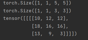
The input image is multiplied and added corresponding to the convolution kernel (Strive=1)

import torch
import torch.nn.functional as F

input = torch.tensor([[1, 2, 0, 3, 1], [0, 1, 2, 3, 1],
                      [1, 2, 1, 0, 0], [5, 2, 3, 1, 1],
                      [2, 1, 0, 1, 1]])

kernel = torch.tensor([[1, 2, 1],
                       [0, 1, 0],
                       [2, 1, 0]])
#Format conversion
input = torch.reshape(input, (1, 1, 5, 5))  # size is 1,5x5
kernel = torch.reshape(kernel, (1, 1, 3, 3))

print(input.shape)
print(kernel.shape)  # Check the size and know that there are only height and width. If it does not meet the requirement of 4 arrays, it needs to be transformed

output = F.conv2d(input, kernel, stride=1)#Two dimensional convolution
print(output)

padding=1: fill a grid


1	2	0	3	1
0	1	2	3	1
1	2	1	0	0
5	2	3	1	1
2	1	0	1	1

out_channels=2 means two channels. Use two convolution kernels to compare the same input image, get two arrays, and then output the results. In fact, many algorithms are increasing the number of channels

Pooling

maxpool maximization is also called downsampling

maxunpool maximization is also called upsampling

Interpretation – a parameter that controls the stripe of elements in the window void convolution, which is different from ordinary convolution and has gaps

ceil_mode – when True, will use ceil instead of floor to compute the output shape

Usage of cell, round up (i.e. keep)

Maximum pooling (maximum output)

Input image:

1	2	0	3	1
0	1	2	3	1
1	2	1	0	0
5	2	3	1	1
2	1	0	1	1

Pooled core (3x3),kernel_size=3

Ceil_model=True

The output result is

2	3
5	1

Ceil_model=false

The output is 2

Maximum pooling function: retain the maximum characteristics of input and reduce the amount of data

In many networks, after one layer of convolution, another layer of pooling, and then nonlinear activation

Nonlinear activation function

inplace is the difference between occupied and unoccupied

Nonlinear transformation mainly introduces some nonlinear characteristics. The more nonlinearity, the better. It conforms to various curves or models with various characteristics

Regularization

Function: it can speed up training

import torch
import torchvision
from torch import nn
from torch.nn import Linear
from torch.utils.data import DataLoader

dataset=torchvision.datasets.CIFAR10("./dataset",train=False,transform=torchvision.transforms.ToTensor(),download=True)

dataloader=DataLoader(dataset,batch_size=64)

class Yjh(nn.Module):

    def __init__(self):
        super().__init__()
        self.linear1=Linear(196608,10)

    def forward(self,input):
        output=self.linear1(input)
        return output

yjh=Yjh()


for data in dataloader:
    imgs,targets=data
    
    output=torch.reshape(imgs,(1,1,1,-1))
    print(output.shape)
    
    output=yjh(output)
    print(output.shape)
    
    The output result is:
    torch.Size([1, 1, 1, 10])
torch.Size([1, 1, 1, 196608])
torch.Size([1, 1, 1, 10])
torch.Size([1, 1, 1, 196608])
torch.Size([1, 1, 1, 10])
torch.Size([1, 1, 1, 196608])
torch.Size([1, 1, 1, 10])
torch.Size([1, 1, 1, 196608])
torch.Size([1, 1, 1, 10])
torch.Size([1, 1, 1, 196608])
torch.Size([1, 1, 1, 10])
torch.Size([1, 1, 1, 196608])
torch.Size([1, 1, 1, 10])
torch.Size([1, 1, 1, 196608])
torch.Size([1, 1, 1, 10])
torch.Size([1, 1, 1, 196608])
torch.Size([1, 1, 1, 10])
torch.Size([1, 1, 1, 196608])
torch.Size([1, 1, 1, 10])
torch.Size([1, 1, 1, 196608])
torch.Size([1, 1, 1, 10])
torch.Size([1, 1, 1, 196608])
torch.Size([1, 1, 1, 10])
torch.Size([1, 1, 1, 196608])
torch.Size([1, 1, 1, 10])
torch.Size([1, 1, 1, 49152])
..........................
..........................

It is obvious that the amount of data is greatly reduced

Turn data into a row

import torch
import torchvision
from torch import nn
from torch.nn import Linear
from torch.utils.data import DataLoader

dataset=torchvision.datasets.CIFAR10("./dataset",train=False,transform=torchvision.transforms.ToTensor(),download=True)

dataloader=DataLoader(dataset,batch_size=64)

class Yjh(nn.Module):

    def __init__(self):
        super().__init__()
        self.linear1=Linear(196608,10)

    def forward(self,input):
        output=self.linear1(input)
        return output

yjh=Yjh()


for data in dataloader:
    imgs,targets=data
    output=torch.flatten(imgs)
    print(output.shape)
    output=yjh(output)
    print(output.shape)
    
    
  #  Output as
torch.Size([196608])
torch.Size([10])
torch.Size([196608])
torch.Size([10])
torch.Size([196608])
torch.Size([10])
torch.Size([196608])
torch.Size([10])
torch.Size([196608])
torch.Size([10])
torch.Size([196608])
torch.Size([10])
................
...............

Sequential use

import torch
from torch import nn
from torch.nn import Conv2d, MaxPool2d, Flatten, Linear, Sequential


class Yjh(nn.Module):
    def __init__(self):
        super().__init__()
        self.conv1 = Conv2d(3, 32, 5, 1, padding=2)
        self.maxpool1 = MaxPool2d(2)
        self.conv2 = Conv2d(32, 32, 5, 1, padding=2)
        self.maxpool2 = MaxPool2d(2)
        self.conv3 = Conv2d(32, 64, 5, padding=2)
        self.maxpool3 = MaxPool2d(2)
        self.flatten = Flatten()
        self.linear1 = Linear(1024, 64)#If you don't know the first parameter, Flatten it with the Flatten function
        self.linear2 = Linear(64, 10)
        
    def forward(self, x):
        x = self.conv1(x)
        x = self.maxpool1(x)
        x = self.conv2(x)
        x = self.maxpool2(x)
        x = self.conv3(x)
        x = self.maxpool3(x)
        x = self.flatten(x)
        x = self.linear1(x)
        x = self.linear2(x)
        return x


yjh = Yjh()
print(yjh)
input = torch.ones((64, 3, 32, 32))
output = yjh(input)
print(output.shape)

Output results:

  (conv1): Conv2d(3, 32, kernel_size=(5, 5), stride=(1, 1), padding=(2, 2))
  (maxpool1): MaxPool2d(kernel_size=2, stride=2, padding=0, dilation=1, ceil_mode=False)
  (conv2): Conv2d(32, 32, kernel_size=(5, 5), stride=(1, 1), padding=(2, 2))
  (maxpool2): MaxPool2d(kernel_size=2, stride=2, padding=0, dilation=1, ceil_mode=False)
  (conv3): Conv2d(32, 64, kernel_size=(5, 5), stride=(1, 1), padding=(2, 2))
  (maxpool3): MaxPool2d(kernel_size=2, stride=2, padding=0, dilation=1, ceil_mode=False)
  (flatten): Flatten(start_dim=1, end_dim=-1)
  (linear1): Linear(in_features=1024, out_features=64, bias=True)
  (linear2): Linear(in_features=64, out_features=10, bias=True)
)
torch.Size([64, 10])

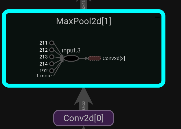
Sequential

import torch
from torch import nn
from torch.nn import Conv2d, MaxPool2d, Flatten, Linear, Sequential
from torch.utils.tensorboard import SummaryWriter


class Yjh(nn.Module):
    def __init__(self):
        super().__init__()
        self.model1=Sequential(
            Conv2d(3, 32, 5, 1, padding=2),#Note that it needs to be separated by commas
            MaxPool2d(2),
            Conv2d(32, 32, 5, 1, padding=2),
            MaxPool2d(2),
            Conv2d(32, 64, 5, padding=2),
            MaxPool2d(2),
            Flatten(),
            Linear(1024, 64),
            Linear(64, 10)
        )

    def forward(self, x):
        x=self.model1(x)
        return x

yjh = Yjh()
print(yjh)
input = torch.ones((64, 3, 32, 32))
output = yjh(input)
print(output.shape)

writer=SummaryWriter("./logs_seq")
writer.add_graph(yjh,input)#Output chart
writer.close()

Output results:

Yjh(
  (model1): Sequential(
  #The serial number is in front
    (0): Conv2d(3, 32, kernel_size=(5, 5), stride=(1, 1), padding=(2, 2))
    (1): MaxPool2d(kernel_size=2, stride=2, padding=0, dilation=1, ceil_mode=False)
    (2): Conv2d(32, 32, kernel_size=(5, 5), stride=(1, 1), padding=(2, 2))
    (3): MaxPool2d(kernel_size=2, stride=2, padding=0, dilation=1, ceil_mode=False)
    (4): Conv2d(32, 64, kernel_size=(5, 5), stride=(1, 1), padding=(2, 2))
    (5): MaxPool2d(kernel_size=2, stride=2, padding=0, dilation=1, ceil_mode=False)
    (6): Flatten(start_dim=1, end_dim=-1)
    (7): Linear(in_features=1024, out_features=64, bias=True)
    (8): Linear(in_features=64, out_features=10, bias=True)
  )
)
torch.Size([64, 10])

tensorboard displays the results

Double click to open

Loss function loss

calculation error
Back propagation, optimization parameters

import torch
from torch import nn
from torch.nn import L1Loss

input = torch.tensor([1, 2, 3], dtype=torch.float32)
targets = torch.tensor([1, 2, 5], dtype=torch.float32)
inputs = torch.reshape(input, (1, 1, 1, 3))  # batch_size,1channel,1 row, 3 columns
targets = torch.reshape(targets, (1, 1, 1, 3), )

loss = L1Loss()#The default is average, which can be sum
result = loss(inputs, targets)
print(result)#|((1-1)+(1-1)+(5-3))/3|=0.667

loss = L1Loss(reduction="sum")
result = loss(inputs, targets)
print(result)

loss_mes=nn.MSELoss()#Square difference
result_mse=loss_mes(inputs,targets)
print(result_mse)#(0+0+2)**2/3

x=torch.tensor([0.1,0.2,0.3])
y=torch.tensor([1])
x=torch.reshape(x,(1,3))#batch_ Size = class 1,3
loss_cross=nn.CrossEntropyLoss()#Cross entropy
result_cross=loss_cross(x,y)#loss(x,class)=-0.2+ln(exp(0.1)+exp(0.2)+exp(0.3))
print(result_cross)

Output results:

tensor(0.6667)
tensor(2.)
tensor(1.3333)
tensor(1.1019)

Calculation formula of cross entropy( Detailed explanation of calculation process)

import torchvision
from torch import nn
from torch.nn import Linear, Flatten, MaxPool2d, Conv2d, Sequential
from torch.utils.data import DataLoader

dataset=torchvision.datasets.CIFAR10("./dataset",train=False,transform=torchvision.transforms.ToTensor())
dataloader=DataLoader(dataset,batch_size=64,shuffle=True)
class Yjh(nn.Module):
    def __init__(self):
        super().__init__()
        self.model1=Sequential(
            Conv2d(3, 32, 5, 1, padding=2),#Note that it needs to be separated by commas
            MaxPool2d(2),
            Conv2d(32, 32, 5, 1, padding=2),
            MaxPool2d(2),
            Conv2d(32, 64, 5, padding=2),
            MaxPool2d(2),
            Flatten(),
            Linear(1024, 64),
            Linear(64, 10)
        )

    def forward(self, x):
        x=self.model1(x)
        return x
loss=nn.CrossEntropyLoss()
yjh=Yjh()
for data in dataloader:
    imgs,targets=data
    outputs=yjh(imgs)
    result_loss=loss(outputs,targets)
    print(result_loss)

Output results:

The following number is the error between the output of the neural network and the real output

tensor(2.3062, grad_fn=<NllLossBackward0>)
tensor(2.2851, grad_fn=<NllLossBackward0>)
tensor(2.2950, grad_fn=<NllLossBackward0>)
tensor(2.3109, grad_fn=<NllLossBackward0>)
tensor(2.3065, grad_fn=<NllLossBackward0>)
tensor(2.3187, grad_fn=<NllLossBackward0>)
tensor(2.3177, grad_fn=<NllLossBackward0>)
tensor(2.3050, grad_fn=<NllLossBackward0>)
tensor(2.2990, grad_fn=<NllLossBackward0>)
tensor(2.3180, grad_fn=<NllLossBackward0>)
tensor(2.2940, grad_fn=<NllLossBackward0>)
tensor(2.3002, grad_fn=<NllLossBackward0>)
tensor(2.2984, grad_fn=<NllLossBackward0>)

optimizer

After debugging, click YJH / protected attributes/_ modules/model1//Protected Attributes/_ grad under modules /'0 '/ weight is the gradient

import torch
import torchvision
from torch import nn
from torch.nn import Linear, Flatten, MaxPool2d, Conv2d, Sequential
from torch.utils.data import DataLoader

dataset = torchvision.datasets.CIFAR10("./dataset", train=False, transform=torchvision.transforms.ToTensor())
dataloader = DataLoader(dataset, batch_size=64, shuffle=True)


class Yjh(nn.Module):
    def __init__(self):
        super().__init__()
        self.model1 = Sequential(
            Conv2d(3, 32, 5, 1, padding=2),  # Note that it needs to be separated by commas
            MaxPool2d(2),
            Conv2d(32, 32, 5, 1, padding=2),
            MaxPool2d(2),
            Conv2d(32, 64, 5, padding=2),
            MaxPool2d(2),
            Flatten(),
            Linear(1024, 64),
            Linear(64, 10)
        )

    def forward(self, x):
        x = self.model1(x)
        return x


loss = nn.CrossEntropyLoss()
yjh = Yjh()
optim = torch.optim.SGD(yjh.parameters(), lr=0.01)  # Don't set the learning rate too high
for epoch in range(20):#Learn all 20 times, usually hundreds or thousands
    running_loss=0.0
    for data in dataloader:
        imgs, targets = data
        outputs = yjh(imgs)
        result_loss = loss(outputs, targets)
        optim.zero_grad()  # Gradient clearing
        result_loss.backward()
        optim.step()
        running_loss=running_loss+result_loss
    print(running_loss)#Overall error

Output results:

tensor(360.1394, grad_fn=<AddBackward0>)
tensor(354.0514, grad_fn=<AddBackward0>)
tensor(330.8956, grad_fn=<AddBackward0>)
tensor(314.3040, grad_fn=<AddBackward0>)
tensor(303.5132, grad_fn=<AddBackward0>)
tensor(295.3024, grad_fn=<AddBackward0>)
tensor(287.8922, grad_fn=<AddBackward0>)
tensor(279.0746, grad_fn=<AddBackward0>)
tensor(273.7878, grad_fn=<AddBackward0>)
tensor(267.6326, grad_fn=<AddBackward0>)
tensor(261.7827, grad_fn=<AddBackward0>)
tensor(256.1693, grad_fn=<AddBackward0>)
tensor(251.1363, grad_fn=<AddBackward0>)
tensor(247.0008, grad_fn=<AddBackward0>)
tensor(242.6788, grad_fn=<AddBackward0>)
tensor(238.7857, grad_fn=<AddBackward0>)
tensor(234.5486, grad_fn=<AddBackward0>)
tensor(231.1932, grad_fn=<AddBackward0>)
tensor(227.9656, grad_fn=<AddBackward0>)
tensor(224.6279, grad_fn=<AddBackward0>)

VGG model

Generally, it is used as a network in front, and then other network models are added later

View network structure

import torchvision
from torch import nn

vgg16_false=torchvision.models.vgg16(pretrained=False)#Untrained = false is untrained, and progress displays the progress bar
vgg16_true=torchvision.models.vgg16(pretrained=True)#Progress displays the progress bar
print(vgg16_false)
train_data=torchvision.datasets.CIFAR10('./dataset',train=True,transform=torchvision.transforms.ToTensor())
vgg16_true.classifier.add_module('add_linear',nn.Linear(1000,10))#The linear model can be added to the sequential of the classifier
print(vgg16_true)
vgg16_false.classifier[6]=nn.Linear(4096,10)#Change the output from 1000 to 10

Output results:

VGG(
  (features): Sequential(
    (0): Conv2d(3, 64, kernel_size=(3, 3), stride=(1, 1), padding=(1, 1))
    (1): ReLU(inplace=True)
    (2): Conv2d(64, 64, kernel_size=(3, 3), stride=(1, 1), padding=(1, 1))
    (3): ReLU(inplace=True)
    (4): MaxPool2d(kernel_size=2, stride=2, padding=0, dilation=1, ceil_mode=False)
    (5): Conv2d(64, 128, kernel_size=(3, 3), stride=(1, 1), padding=(1, 1))
    (6): ReLU(inplace=True)
    (7): Conv2d(128, 128, kernel_size=(3, 3), stride=(1, 1), padding=(1, 1))
    (8): ReLU(inplace=True)
    (9): MaxPool2d(kernel_size=2, stride=2, padding=0, dilation=1, ceil_mode=False)
    (10): Conv2d(128, 256, kernel_size=(3, 3), stride=(1, 1), padding=(1, 1))
    (11): ReLU(inplace=True)
    (12): Conv2d(256, 256, kernel_size=(3, 3), stride=(1, 1), padding=(1, 1))
    (13): ReLU(inplace=True)
    (14): Conv2d(256, 256, kernel_size=(3, 3), stride=(1, 1), padding=(1, 1))
    (15): ReLU(inplace=True)
    (16): MaxPool2d(kernel_size=2, stride=2, padding=0, dilation=1, ceil_mode=False)
    (17): Conv2d(256, 512, kernel_size=(3, 3), stride=(1, 1), padding=(1, 1))
    (18): ReLU(inplace=True)
    (19): Conv2d(512, 512, kernel_size=(3, 3), stride=(1, 1), padding=(1, 1))
    (20): ReLU(inplace=True)
    (21): Conv2d(512, 512, kernel_size=(3, 3), stride=(1, 1), padding=(1, 1))
    (22): ReLU(inplace=True)
    (23): MaxPool2d(kernel_size=2, stride=2, padding=0, dilation=1, ceil_mode=False)
    (24): Conv2d(512, 512, kernel_size=(3, 3), stride=(1, 1), padding=(1, 1))
    (25): ReLU(inplace=True)
    (26): Conv2d(512, 512, kernel_size=(3, 3), stride=(1, 1), padding=(1, 1))
    (27): ReLU(inplace=True)
    (28): Conv2d(512, 512, kernel_size=(3, 3), stride=(1, 1), padding=(1, 1))
    (29): ReLU(inplace=True)
    (30): MaxPool2d(kernel_size=2, stride=2, padding=0, dilation=1, ceil_mode=False)
  )
  (avgpool): AdaptiveAvgPool2d(output_size=(7, 7))
  (classifier): Sequential(
    (0): Linear(in_features=25088, out_features=4096, bias=True)
    (1): ReLU(inplace=True)
    (2): Dropout(p=0.5, inplace=False)
    (3): Linear(in_features=4096, out_features=4096, bias=True)
    (4): ReLU(inplace=True)
    (5): Dropout(p=0.5, inplace=False)
    (6): Linear(in_features=4096, out_features=1000, bias=True)
  )
)
VGG(
  (features): Sequential(
    (0): Conv2d(3, 64, kernel_size=(3, 3), stride=(1, 1), padding=(1, 1))
    (1): ReLU(inplace=True)
    (2): Conv2d(64, 64, kernel_size=(3, 3), stride=(1, 1), padding=(1, 1))
    (3): ReLU(inplace=True)
    (4): MaxPool2d(kernel_size=2, stride=2, padding=0, dilation=1, ceil_mode=False)
    (5): Conv2d(64, 128, kernel_size=(3, 3), stride=(1, 1), padding=(1, 1))
    (6): ReLU(inplace=True)
    (7): Conv2d(128, 128, kernel_size=(3, 3), stride=(1, 1), padding=(1, 1))
    (8): ReLU(inplace=True)
    (9): MaxPool2d(kernel_size=2, stride=2, padding=0, dilation=1, ceil_mode=False)
    (10): Conv2d(128, 256, kernel_size=(3, 3), stride=(1, 1), padding=(1, 1))
    (11): ReLU(inplace=True)
    (12): Conv2d(256, 256, kernel_size=(3, 3), stride=(1, 1), padding=(1, 1))
    (13): ReLU(inplace=True)
    (14): Conv2d(256, 256, kernel_size=(3, 3), stride=(1, 1), padding=(1, 1))
    (15): ReLU(inplace=True)
    (16): MaxPool2d(kernel_size=2, stride=2, padding=0, dilation=1, ceil_mode=False)
    (17): Conv2d(256, 512, kernel_size=(3, 3), stride=(1, 1), padding=(1, 1))
    (18): ReLU(inplace=True)
    (19): Conv2d(512, 512, kernel_size=(3, 3), stride=(1, 1), padding=(1, 1))
    (20): ReLU(inplace=True)
    (21): Conv2d(512, 512, kernel_size=(3, 3), stride=(1, 1), padding=(1, 1))
    (22): ReLU(inplace=True)
    (23): MaxPool2d(kernel_size=2, stride=2, padding=0, dilation=1, ceil_mode=False)
    (24): Conv2d(512, 512, kernel_size=(3, 3), stride=(1, 1), padding=(1, 1))
    (25): ReLU(inplace=True)
    (26): Conv2d(512, 512, kernel_size=(3, 3), stride=(1, 1), padding=(1, 1))
    (27): ReLU(inplace=True)
    (28): Conv2d(512, 512, kernel_size=(3, 3), stride=(1, 1), padding=(1, 1))
    (29): ReLU(inplace=True)
    (30): MaxPool2d(kernel_size=2, stride=2, padding=0, dilation=1, ceil_mode=False)
  )
  (avgpool): AdaptiveAvgPool2d(output_size=(7, 7))
  (classifier): Sequential(
    (0): Linear(in_features=25088, out_features=4096, bias=True)
    (1): ReLU(inplace=True)
    (2): Dropout(p=0.5, inplace=False)
    (3): Linear(in_features=4096, out_features=4096, bias=True)
    (4): ReLU(inplace=True)
    (5): Dropout(p=0.5, inplace=False)
    (6): Linear(in_features=4096, out_features=1000, bias=True)
    (add_linear): Linear(in_features=1000, out_features=10, bias=True)
  )
)

Model saving

import torch
import torchvision.models
vgg16 = torchvision.models.vgg16(pretrained=False)
# Save method 1 is best saved as pth, which not only saves the network model structure, but also saves the parameters
torch.save(vgg16, "vgg16_methd1.pth")
# Save method 2 saves the parameters in the network model in the form of Dictionary (official recommendation), with small space
torch.save(vgg16.state_dict(), 'vgg16_methd2.pth')

Model loading

import torch
#Loading method corresponding to saving method 1
import torchvision.models

model=torch.load("vgg16_methd1.pth")#If you use your own network model, you need to redefine the class when loading
print(model)

#Loading method corresponding to saving method 2
#Restore network model structure
vgg16=torchvision.models.vgg16(pretrained=False)
vgg16.load_state_dict("vgg16_methd2.pth")
# model2=torch.load("vgg16_methd1.pth")
print(vgg16)

Complete model training routine

import torch
import torchvision
from torch import nn
from torch.utils.data import DataLoader
from torch.utils.tensorboard import SummaryWriter

from model import *  # Import everything from another file

# Prepare training set


train_data = torchvision.datasets.CIFAR10("./dataset", train=True, download=True,
                                          transform=torchvision.transforms.ToTensor())

test_data = torchvision.datasets.CIFAR10("./dataset", train=False, transform=torchvision.transforms.ToTensor(),
                                         download=True)

# length
train_data_size = len(train_data)
test_data_size = len(test_data)
print("The length of the training set is:{}".format(train_data_size))
print("The length of the test set is:{}".format(test_data_size))

# Load training set
train_dataloader = DataLoader(train_data, batch_size=64, shuffle=True)
test_dataloader = DataLoader(test_data, batch_size=64, shuffle=True)

# Create network model
yjh = Yjh()

# loss function 
loss_fn = nn.CrossEntropyLoss()

# optimizer
learning_rate = 1e-2  # I'm used to extracting this parameter
optimizer = torch.optim.SGD(yjh.parameters(), lr=learning_rate, )  # gradient descent 

# Set some parameters of the training network
total_train_step = 0  # Record the number of workouts
total_test_step = 0  # Record the number of tests
epoch = 10  # Number of rounds of training

# Add tensorboard
writer = SummaryWriter("./logs_train_1")

for i in range(epoch):
    print("-----The first{}Round of training begins-----".format(i + 1))
    yjh.train()#Set the network to training mode and work on specific layers
    for data in train_dataloader:
        imgs, targets = data
        output = yjh(imgs)
        loss = loss_fn(output, targets)
        # Optimizer optimization model
        optimizer.zero_grad()
        loss.backward()
        optimizer.step()
        total_train_step += 1
        if total_train_step % 100 == 0:
            print("Training times:{},Loss={}".format(total_train_step, loss.item()))  # Finally, adding item () will directly output a number. Finally, it can also be written directly as loss
            writer.add_scalar("train_loss", loss.item(), total_train_step)

    # testing procedure
    yjh.eval()#Set the network to authentication mode to work on a specific layer
    total_accuracy=0#Overall accuracy
    total_test_loss = 0  # Calculate the error of the entire data set
    with torch.no_grad():#No gradient is set, and there is no need to change the gradient
        for data in test_dataloader:
            imgs, targets = data
            outputs = yjh(imgs)
            loss = loss_fn(outputs, targets)
            total_test_loss = total_test_loss + loss.item()
            accuracy=(outputs.argmax(1)==targets).sum()
            total_accuracy=total_accuracy+accuracy
    print("On the overall test set Loss:{}".format(total_test_loss))
    print("Accuracy on the overall test set:{}".format(total_accuracy/test_data_size))
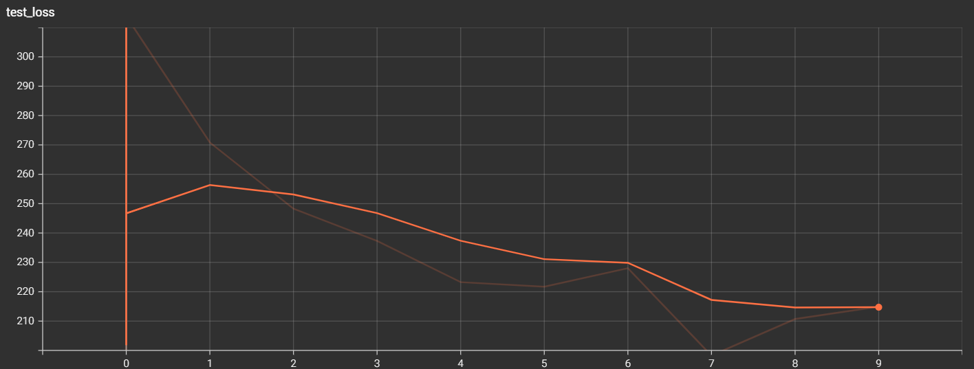
    writer.add_scalar("test_loss", total_test_loss, total_test_step)
    writer.add_scalar("Test accuracy",total_accuracy/test_data_size,total_test_step)
    total_test_step += 1

#Save model
    torch.save(yjh,"yjh_{}.pth".format(i))#Save several rounds of training model
    #torch.save(yjh.state_dict(),"yjh_{}.pth".farmat(1))#Official recommendation
    print("Model saved")
writer.close()

The model is placed separately py

import torch
from torch import nn
from model import *

class Yjh(nn.Module):
    def __init__(self) -> None:
        super().__init__()
        self.model = nn.Sequential(
            nn.Conv2d(in_channels=3, out_channels=32, kernel_size=5, stride=1, padding=2),
            nn.MaxPool2d(2),
            nn.Conv2d(32, 32, kernel_size=5, stride=1, padding=2),
            nn.MaxPool2d(2),
            nn.Conv2d(32, 64, kernel_size=5, stride=1, padding=2),
            nn.MaxPool2d(2),
            nn.Flatten(),
            nn.Linear(1024, 64),
            nn.Linear(64, 10)
        )

    def forward(self, x):
        x = self.model(x)
        return x

if __name__ == '__main__':
    yjh = Yjh()
    input = torch.ones((64, 3, 32, 32))
    output = yjh(input)
    print(output.shape)

Output results:

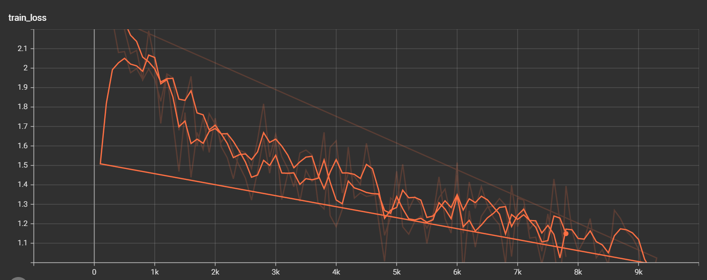
Note: the irregular descent curve is the correct output

It can be seen from the above figure that the more model training, the lower the loss of the model

Accuracy judgment of model

2xinput

Model(2 classification)

output=[0.1,0.2] [0.3,0.4]

Get the maximum probability through Argmax, i.e. Preds=[1] [1]

input target=[0] [1]

Preds==inputs target

[false,true].sum()=1

Code implementation:

import torch

outputs = torch.tensor([[0.1, 0.2], [0.3, 0.4]])
print(outputs.argmax(1))#If the value is 1, the horizontal ratio is compared, such as 0.1 and 0.2, and if the value is 0, the vertical ratio is compared, such as 0.1 and 0.3

preds=outputs.argmax(1)
targets=torch.tensor([0,1])
print((preds==targets).sum())

Output results:

tensor([1, 1])
tensor(1)

GPU training (much faster than CPU)

Method 1: realize the following four conditions

network model

yjh = Yjh()
if torch.cuda.is_available():
    yjh=yjh.cuda()#Transfer the network model to cuda

Data (input, output)

imgs, targets = data
if torch.cuda.is_available():
    imgs=imgs.cuda()
    targets=targets.cuda()

loss function

# loss function 
loss_fn = nn.CrossEntropyLoss()
if torch.cuda.is_available():#Determine whether the GPU is available
    loss_fn=loss_fn.cuda()

.cuda()

Time taken for 400 times under GPU training:

The time for training 200 is:9.526910781860352
 Training times: 200,Loss=2.2695932388305664
 The time of training 400 is:11.822770833969116
 Training times: 400,Loss=2.1631038188934326

Time spent training 400 times without GPU

The time for training 200 is:12.44710397720337
 Training times: 200,Loss=2.2931666374206543
 The time of training 400 is:24.154792308807373
 Training times: 400,Loss=2.231562852859497

If there is no hardware GPU, you can use Google's collab to create a new notebook, and then set GPU acceleration in the notebook settings in the file, which can be used for free 30 hours a week (very fast)

Mode 2: it is easy to change the configuration uniformly
1. First define a device: device = torch device(“cuda”)
  
  If there are multiple, you can also specify a graphics card torch device(“cuda:1”)
2. Similar to mode 1, in Used at cuda() to(device)
  
  as
```
if torch.cuda.is_available():#Determine whether the GPU is available
    loss_fn=loss_fn.to(device)
```

Model validation

By adding breakpoints when adding data sets and checking the classification index after debug ging, you can get the following pictures

import torch
import torchvision.transforms
from PIL import Image
from torch import nn

image_path = "./imgs/img_1.png"
image = Image.open(image_path)

image = image.convert("RGB")  # Because png is four channel, it needs to be changed to three channel
transform = torchvision.transforms.Compose([torchvision.transforms.Resize((32, 32)), torchvision.transforms.ToTensor()])
image = transform(image)
print(image.shape)

# Create network model
class Yjh(nn.Module):
    def __init__(self) -> None:
        super().__init__()
        self.model = nn.Sequential(
            nn.Conv2d(in_channels=3, out_channels=32, kernel_size=5, stride=1, padding=2),
            nn.MaxPool2d(2),
            nn.Conv2d(32, 32, kernel_size=5, stride=1, padding=2),
            nn.MaxPool2d(2),
            nn.Conv2d(32, 64, kernel_size=5, stride=1, padding=2),
            nn.MaxPool2d(2),
            nn.Flatten(),
            nn.Linear(1024, 64),
            nn.Linear(64, 10)
        )

    def forward(self, x):
        x = self.model(x)
        return x

model = torch.load("yjh_0.pth", map_location=torch.device("cpu"))  # Pay attention to how the model trained on GPU runs when loading
print(model)
image=torch.reshape(image, (1, 3, 32, 32))
model.eval()
with torch.no_grad():  # Available without gradient, save memory and improve performance
    output = model(image)
print(output)
print(output.argmax(1))

Output is:

tensor([[ 1.2021,  0.4194,  0.0154, -0.8249, -0.9728, -0.7813, -1.5403, -0.3458,
          1.6731,  1.2716]])
tensor([8])

The result is not correct, because the model has only undergone one round of training

model = torch.load("yjh_49.pth", map_location=torch.device("cpu"))  # When loading the model trained on GPU, pay attention to how to run it. Load the model trained 50 times

The output result is

tensor([[  3.7672, -25.3946,   7.4116,  10.2170,   1.1890,  11.3926,   7.7192,
          -0.6535,  -4.2947, -10.5369]])
tensor([5])

The result is correct

stay Introduction to pytorch video In the middle school, the small mound has achieved nanny level teaching, and many important places have repeatedly mentioned that the teaching content and methods are not boring. Compared with other pytorch introductory videos I have seen, the video of the small mound has really achieved introductory teaching, rather than persuading the teaching. If you follow the small mound step by step, you will find it more and more interesting, with complete content and reasonable arrangement, The front row recommends students who want to learn pytorch to watch. In case of errors, small mounds will patiently find and teach how to find and solve errors. In the process of learning pytorch, they have also learned a lot of other knowledge. Why not! In their own practice, there is an error that the teacher does not appear. Don't worry. Baidu can easily solve it!

Topics: Python Pytorch Deep Learning

Programmer Think

Introduction notes to pytorch

Use of TensorBoard (one data)

torchvision uniformly manages and processes data sets

dataload (load partial data from dataset)

nn.Module neural network basic skeleton

debugging

Convolution use

Pooling

Regularization

Sequential use

Loss function loss

optimizer

Model saving

Model loading

Complete model training routine

Accuracy judgment of model

GPU training (much faster than CPU)

Model validation

Hot Topics