Introduction of ConvGRU neural network

1. Introduction to convolutional neural network

• Convolutional neural network is a deep feedforward neural network with the characteristics of local connection and weight sharing

  • characteristic:

    • Local connection:
      • In the convolution layer, each neuron is only connected with the neuron in a local window in the previous layer to form a local neural network
    • Weight sharing
      • Convolution kernel of parameters w ( l ) w^{(l)} w(l) is the same for all neurons in layer l
    • Convergence

  • Advantages: translation, scaling, rotation invariance

  • Composition: at present, convolutional neural network is generally composed of convolution layer, convergence layer and full connection layer

    • Convolution layer:
      • Different convolution kernels are equivalent to different feature extractors to extract the features of local regions
      • Feature mapping: input the features extracted by convolution, and each feature mapping can be used as a class of extracted image features

  • Program implementation:

    • In pytorch, the implementation of convolution layer is to load torch nn. NN
    • The calling function is NN conv2D
      • in_channels: number of channels entered
      • out_channels: number of output channels
      • kernel_size: convolution kernel size
      • Stripe: step size
      • Padding: controls the number of zero padding
    • Input / output Description:
      • The dimension of the input variable should be (batch_size, in_channels, width, length)
      • The output is

import torch 
import torch.nn as nn
conv = nn.Conv2d(in_channels=1,out_channels =16, kernel_size=3, stride =1)
inputs = torch.randn(1, 1, 64, 64) #(sampltNum, channels, width, length)
out = conv(inputs)

2. Recurrent neural network

• GRU neural network is a kind of cyclic neural network and a variant of LSTM. Based on LSTM neural network, cell structure is optimized, parameters are reduced and training speed is accelerated;

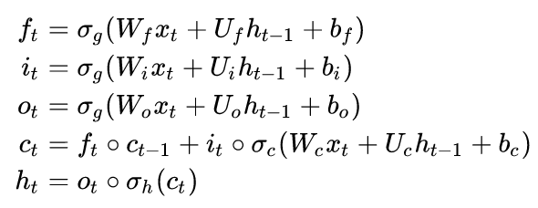
• The calculation formula of LSTM is:

  • 

  • Where f is the forgetting gate, which determines the degree to which the previous layer is forgotten

  • i is the input gate, which controls how much the new state of the current calculation is updated to the memory cell

  • o is the output gate, which controls how much the current output depends on the current memory unit

  • c is the memory unit. It can be seen that the cell state is comprehensively calculated by weight, input, hidden layer input of the upper layer, memory unit state of the upper layer and input gate

  • The hidden layer state of this layer is determined by the output gate and memory cell state

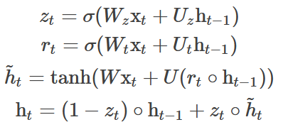
• The calculation formula of GRU is:
  *

  • GRU discards the memory unit in the LSTM and combines the input gate and the forgetting gate into an update gate
  • z is the update gate, which determines how many states of the migration layer need to be updated in the current neuron
  • h ^ \hat{h} h ^ is the candidate value of the hidden layer, but it can be seen from the last function that the candidate value of the hidden layer needs to be calculated and updated by using the update gate

• Implementation of LSTM and GRU

  • The implementation of LSTM and GRU is provided in pytorch
    • parameter
      – input_size
      – hidden_size
      – num_layers
      – bias
      – batch_first
      – dropout
      – bidirectional
    • input
      – input (seq_len, batch, input_size)
      – h_0 (num_layers * num_directions, batch, hidden_size)
      – c_0 (num_layers * num_directions, batch, hidden_size)
    • output
      – output (seq_len, batch, num_directions * hidden_size)
      – h_n (num_layers * num_directions, batch, hidden_size)
      – c_n (num_layers * num_directions, batch, hidden_size)

      rnn = nn.LSTM(input_size=10, hidden_size=20, num_layers=2)#(input_size,hidden_size,num_layers)
      input = torch.randn(5, 3, 10)#(seq_len, batch, input_size)
      h0 = torch.randn(2, 3, 20) #(num_layers,batch,output_size)
      c0 = torch.randn(2, 3, 20) #(num_layers,batch,output_size)
      output, (hn, cn) = rnn(input, (h0, c0))
      

3. Introduction to convgru

ConvGRU is modified according to Dr. Shi's ConvLSTM to convert LSTM into GRU for calculation. ConvLSTM uses convolution kernel to replace the full connection layer in LSTM, that is, the full connection is changed into local connection. GRU is used for comparison and calculation based on torch. The traditional GRU is represented by torch, and the forward propagation process is as follows:

import torch
import torch.nn as nn
import torch.nn.functional as F

def GRU_forward(x, h_t_1):
    """GRU technological process
    args:
        x: input
        h_t_1: Hidden layer output value of the previous layer
    shape: 
        x: [1, feature_size]
        h_t_1: [hidden_size, hidden_size]
    """
    linear_x_z = nn.Linear(10, 5) #(feature_size, hidden_size)
    linear_h_z = nn.Linear(5, 5)  #(hidden_size, hidden_size)
    linear_x_r = nn.Linear(10, 5)
    linear_h_r = nn.Linear(5, 5)
    z_t = F.sigmoid(linear_x_z(x) + linear_h_z(h_t_1))
    r_t = F.sigmoid(linear_x_r(x) + linear_h_r(h_t_1))
    linear = nn.Linear(10,5)
    linear_u = nn.Linear(5,5)
    h_hat_t = F.tanh(linear(x) + linear_u(torch.mul(r_t, h_t_1)))
    h_t = torch.mul((1 - z_t), h_t_1) + torch.mul(z_t, h_hat_t)
    linear_out = nn.Linear(5, 1) #(hidden_size, out_size)
    y = linear_out(h_t)
    return y, h_t
    
### example ###
x = torch.randn(1,10)
h_t_1 = torch.randn(5,5)

y, h = GRU_forward(x, h_t_1)
    

In convgru, all the above linear layers will be transformed into conv layers, and the input variables will change. The input variables in traditional GRU are two-dimensional variables, while the input variables in convgru are three-dimensional variables. The forward propagation process of convgru is as follows:

def convGru_forward(x, h_t_1):
    """GRU Convolution flow
    args:
        x: input
        h_t_1: Hidden layer output value of the previous layer
    shape: 
        x: [1, channels, width, lenth]
    """
    conv_x_z = nn.Conv2d(
                in_channels=1, out_channels=4, kernel_size=1, stride=1)
    conv_h_z = nn.Conv2d(
                in_channels=4, out_channels=4, kernel_size=1, stride=1)
    z_t = F.sigmoid(conv_x_z(x) + conv_h_z(h_t_1))
    
    conv_x_r = nn.Conv2d(
                in_channels=1, out_channels=4, kernel_size=1, stride=1)
    conv_h_r = nn.Conv2d(
                in_channels=4, out_channels=4, kernel_size=1, stride=1)
    r_t = F.sigmoid((conv_x_r(x) + conv_h_r(h_t_1)))
    
    conv =  nn.Conv2d(
                in_channels=1, out_channels=4, kernel_size=1, stride=1)
    conv_u =  nn.Conv2d(
                in_channels=4, out_channels=4, kernel_size=1, stride=1)
    
    h_hat_t = F.tanh(conv(x) + conv_u(torch.mul(r_t, h_t_1)))
    
    h_t = torch.mul((1 - z_t), h_t_1) + torch.mul(z_t, h_hat_t)
    conv_out = nn.Conv2d(
                in_channels=4, out_channels=1, kernel_size=1, stride=1) #(hidden_size, out_size)
    y = conv_out(h_t)
    return y, h_t
    
x = torch.randn(1, 1, 16,16)
h_t_1 = torch.randn(1, 4, 16, 16)
y_3, h_3 = convGru_forward(x, h_t_1) 
    
print(y_3.size())