This article begins with the official account of "AI little boy".
Last article This paper introduces the basic process of post training quantization, and demonstrates the simplest post training quantization algorithm with pytorch.
Although post training quantization is easy to operate, most reasoning frameworks provide such off-line quantization algorithms (such as tensorrt,ncnn,SNPE But sometimes this method can not guarantee sufficient accuracy. Therefore, this paper introduces another quantization method which is more effective than post training quantization - Quantitative perception training.
Quantitative perception training, as its name suggests, is to train the network in the process of quantization, so that the network parameters can better adapt to the information loss caused by quantization. This method is more flexible, so the accuracy is generally higher than post training quantification. Of course, one of its major disadvantages is inconvenient operation, which will be discussed in detail later.
Similarly, this article will explain the simplest process of quantitative training algorithm, and use the code framework of the previous article to build the process of quantitative training algorithm from zero with pytorch.
Difficulties in quantifying training
To understand the difficulties of quantitative training, we need to understand the difference between quantitative training and ordinary full precision training. To see this clearly, let's review the code of convolutional quantization in the previous article:
class QConv2d(QModule):

    def forward(self, x):
        if hasattr(self, 'qi'):
            self.qi.update(x)

        self.qw.update(self.conv_module.weight.data)

        self.conv_module.weight.data = self.qw.quantize_tensor(self.conv_module.weight.data)
        self.conv_module.weight.data = self.qw.dequantize_tensor(self.conv_module.weight.data)

        x = self.conv_module(x)

        if hasattr(self, 'qo'):
            self.qo.update(x)

        return x
The difference from the full precision model is that we quantify the weight before convolution, and then turn it into float. This step is actually optional in post training quantization, but it is necessary in quantitative perception training. "I added this step in advance for code consistency."
Is there anything special about this step? You can review the specific operation of quantification:
def quantize_tensor(x, scale, zero_point, num_bits=8, signed=False):
    if signed:
        qmin = - 2. ** (num_bits - 1)
        qmax = 2. ** (num_bits - 1) - 1
    else:
        qmin = 0.
        qmax = 2.**num_bits - 1.

    q_x = zero_point + x / scale
    q_x.clamp_(qmin, qmax).round_()

    return q_x.float()
There is a round function in it, and this function cannot be trained. Its function image is as follows:
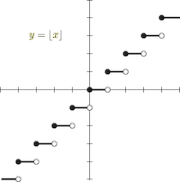
Almost every gradient of this function is 0. If this function exists in the network, the gradient of back propagation will also become 0.
Take an example:
conv = nn.Conv2d(3, 1, 3, 1)

def quantize(weight):
    w = weight.round()
    return w

class QuantConv(nn.Module):

    def __init__(self, conv_module):
        super(QuantConv, self).__init__()
        self.conv_module = conv_module

    def forward(self, x):
        return F.conv2d(x, quantize(self.conv_module.weight), self.conv_module.bias, 3, 1)


x = torch.randn((1, 3, 4, 4))

quantconv = QuantConv(conv)

a = quantconv(x).sum().backward()

print(quantconv.conv_module.weight.grad)
In this example, I perform the round operation on the weight and then perform the convolution operation, but the returned gradients are all 0:
tensor([[[[0., 0., 0.],
          [0., 0., 0.],
          [0., 0., 0.]],

         [[0., 0., 0.],
          [0., 0., 0.],
          [0., 0., 0.]],

         [[0., 0., 0.],
          [0., 0., 0.],
          [0., 0., 0.]]]])
In other words, this function cannot be learned, resulting in the inability of quantitative training.
Straight Through Estimator
How to solve this problem?
An easy way to think of is to skip the pseudo quantization process and avoid round. The gradient of the convolution layer is directly transmitted back to the weight before pseudo quantization. In this way, since the weight used in convolution is operated by pseudo quantization, the quantization error can be simulated, the gradient of these errors can be transmitted back to the original weight, and the weight can be updated to adapt to the error generated by quantization, and the quantization training can be carried out normally.
This method is called Straight Through Estimator(STE).
pytorch implementation
The relevant codes of this article can be found in https://github.com/Jermmy/pytorch-quantization-demo Found on.
Pseudo quantization node implementation
After talking about the basic idea of quantitative training, let's continue to use the previous code framework and add the part of quantitative training.
First, we need to modify the writing method of pseudo quantization. The previous code directly pseudo quantized the value of weight:
self.conv_module.weight.data = self.qw.quantize_tensor(self.conv_module.weight.data)
self.conv_module.weight.data = self.qw.dequantize_tensor(self.conv_module.weight.data)
This is no problem in post training quantization, but in pytorch, this writing method cannot return the gradient. Therefore, in quantization training, the writing method of pseudo quantization node needs to be modified again.
In addition, STE requires us to redefine the gradient of back propagation. Therefore, it is necessary to redefine the pseudo quantization process with the help of the Function interface in pytorch:
from torch.autograd import Function

class FakeQuantize(Function):

    @staticmethod
    def forward(ctx, x, qparam):
        x = qparam.quantize_tensor(x)
        x = qparam.dequantize_tensor(x)
        return x

    @staticmethod
    def backward(ctx, grad_output):
        return grad_output, None
The forward function here is similar to the previous writing method, which is to quantize the value and then inverse quantize it back. But in backward, we directly return the gradient grad passed from the next layer_ Output, which is equivalent to directly skipping the gradient calculation of the pseudo quantization layer and allowing the gradient to flow directly to the previous layer (Straight Through).
pytorch defines that the return variables of the backward function need to correspond to the input parameters of forward, representing the gradient of the corresponding input respectively. Since qparam only counts min and max without gradient, the gradient returned to it is None.
Quantized convolutional code
Except that the pseudo quantization node needs to be modified in forward, the other codes of quantization volume layer are basically the same as those in the previous articles:
class QConv2d(QModule):

    def forward(self, x):
        if hasattr(self, 'qi'):
            self.qi.update(x)
            x = FakeQuantize.apply(x, self.qi)

        self.qw.update(self.conv_module.weight.data)

        x = F.conv2d(x, FakeQuantize.apply(self.conv_module.weight, self.qw),
                     self.conv_module.bias,
                     stride=self.conv_module.stride,
                     padding=self.conv_module.padding, dilation=self.conv_module.dilation,
                     groups=self.conv_module.groups)

        if hasattr(self, 'qo'):
            self.qo.update(x)
            x = FakeQuantize.apply(x, self.qo)

        return x
Because we need to do some pseudo quantization on weight first, according to the rules in pytorch, when doing convolution operation, we can't use x = self as before conv_ Module (x), which should be called by F.conv2d. In addition, there is no pseudo quantization node in the input and output of the previous code, which is no problem in the post training quantization, but it is best to add it in the quantization training to facilitate the network to better perceive the loss caused by quantization.
When I did quantitative reasoning in the last article, I found that the loss of accuracy is not too heavy. In the case of three bit s, the accuracy can still reach 96%. In order to better understand the benefits of quantitative training, we need to be more detailed in the code of quantitative reasoning to increase the quantitative loss:
class QConv2d(QModule):

    def quantize_inference(self, x):
        x = x - self.qi.zero_point
        x = self.conv_module(x)
        x = self.M * x
        x.round_()      # Add one more round operation
        x = x + self.qo.zero_point
        x.clamp_(0., 2.**self.num_bits-1.).round_()
        return x
Compared with the previous code, it actually adds a round to make the quantitative reasoning closer to the real reasoning process.
Quantify the benefits of training
Here we still use the small network in the previous article to test the classification accuracy on mnist. Due to the modification of quantitative reasoning, in order to facilitate comparison, I ran again and trained the accuracy of quantification:
| bit | 1 | 2 | 3 | 4 | 5 | 6 | 7 | 8 |
|---|---|---|---|---|---|---|---|---|
| accuracy | 10% | 47% | 83% | 96% | 98% | 98% | 98% | 98% |
Next, test the effect of quantitative training. The following is the log output when bit=3:
Test set: Full Model Accuracy: 98%

Quantization bit: 3
Quantize Aware Training Epoch: 1 [3200/60000]   Loss: 0.087867
Quantize Aware Training Epoch: 1 [6400/60000]   Loss: 0.219696
Quantize Aware Training Epoch: 1 [9600/60000]   Loss: 0.283124
Quantize Aware Training Epoch: 1 [12800/60000]  Loss: 0.172751
Quantize Aware Training Epoch: 1 [16000/60000]  Loss: 0.315173
Quantize Aware Training Epoch: 1 [19200/60000]  Loss: 0.302261
Quantize Aware Training Epoch: 1 [22400/60000]  Loss: 0.218039
Quantize Aware Training Epoch: 1 [25600/60000]  Loss: 0.301568
Quantize Aware Training Epoch: 1 [28800/60000]  Loss: 0.252994
Quantize Aware Training Epoch: 1 [32000/60000]  Loss: 0.138346
Quantize Aware Training Epoch: 1 [35200/60000]  Loss: 0.203350

...

Test set: Quant Model Accuracy: 90%
The overall experimental results are as follows:
| bit | 1 | 2 | 3 | 4 | 5 | 6 | 7 | 8 |
|---|---|---|---|---|---|---|---|---|
| accuracy | 10% | 63% | 90% | 97% | 98% | 98% | 98% | 98% |
plot them together with a curve:
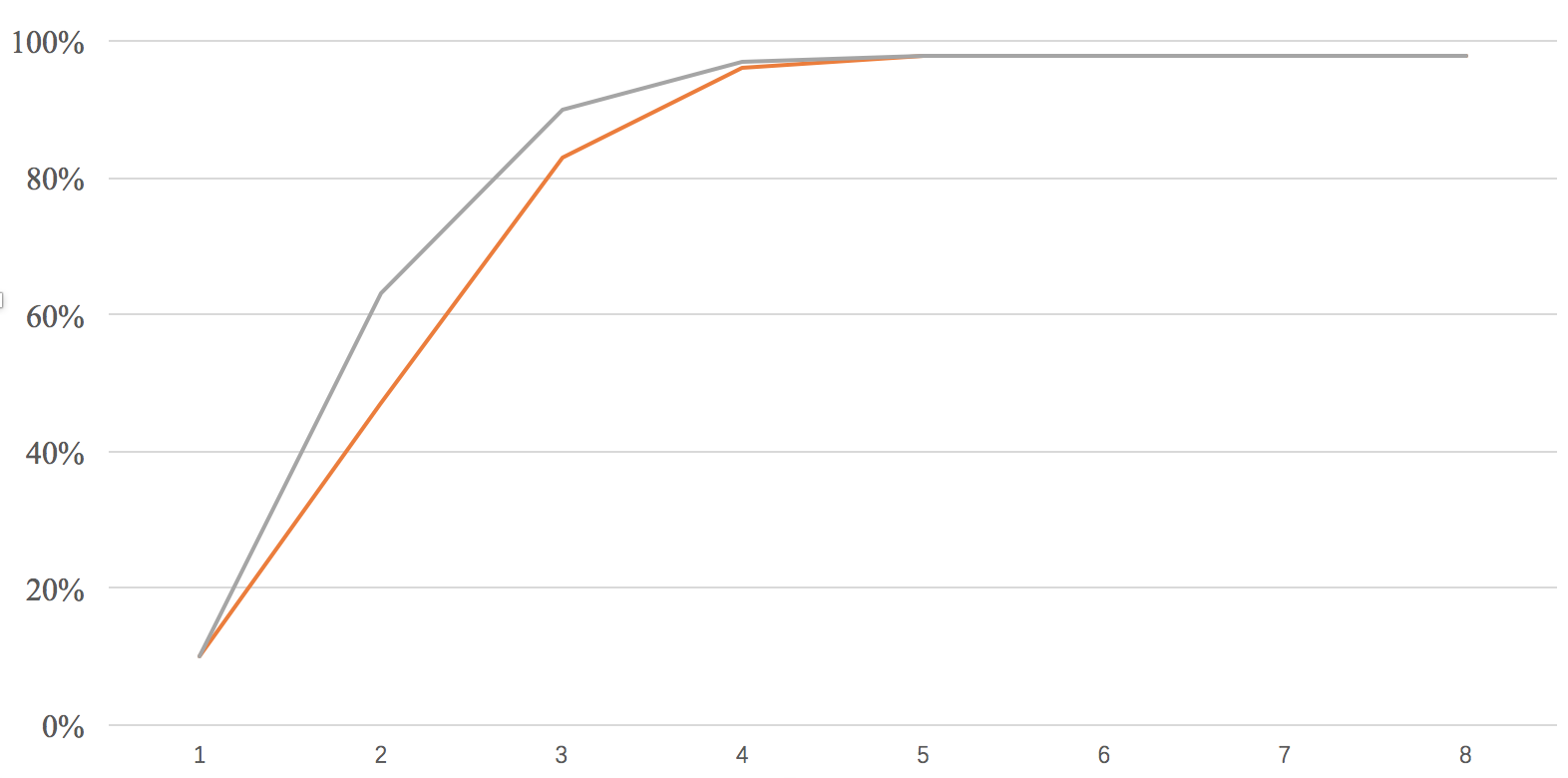
The gray line is quantitative training and the orange line is post training quantification. It can be seen that quantitative training can bring obvious improvement when bit = 2 and 3.
When bit = 1, I found that the gradient of quantization training return is 0, and the training basically failed. This is because when bit = 1, the whole network has degenerated into a binary network, and low bit quantization training itself is not an easy thing. Although we solved the gradient problem with STE earlier, due to the huge information loss of the network due to low bits, the usual training methods are difficult to work.
In addition, there are many trick s in quantization training. In this experiment, I found that the learning rate has a very significant impact on the results. Especially in low bit quantization, the learning rate is too high, which can easily lead to the gradient becoming 0, resulting in the complete failure of quantization training, "once thought the code was wrong".
Quantitative training deployment
As mentioned earlier, although quantitative training has obvious benefits, it is much more troublesome in practical application than post training quantitative training.
At present, when most mainstream reasoning frameworks train quantization after processing, users only need to throw in the model and data to get the quantitative model, and then deploy it directly. However, few frameworks support quantitative training. At present, there is a lack of unified specification for quantitative training. Although the quantitative algorithms of each reasoning engine are the same in essence, it is difficult to achieve consistency in many details. At present, the front-end framework for model training is not unified. "Of course, the mainstream is tf and pytorch". If each reasoning engine needs to support quantitative training of different front-end, it needs to be based on the implementation rules deployed at the back-end according to different front-end frameworks, "such as which layers of quantization need to be merged, whether weight adopts symmetrical quantization, etc.", Build a quantitative training framework from scratch, which is frightening to think about.
summary
This article mainly introduces the basic methods of quantitative training, and constructs a simple quantitative training example with pytorch. The next article will introduce the last article in this series - about fold BatchNorm.