1, Import common libraries
import pandas as pd
import numpy as np
import matplotlib.pyplot as plt
2, Create object
(1) By passing a list to create a Series, pandas will create an integer index by default
The code is as follows:
s = pd.Series([1, 3, 5, np.nan, 6, 8])
print(s)
The operation results are as follows:
0    1.0
1    3.0
2    5.0
3    NaN
4    6.0
5    8.0
dtype: float64
Description: Series: an object similar to one-dimensional array, which is composed of a set of data (various NumPy data types) and a set of related data labels (i.e. indexes). Simple series objects can also be generated from only one set of data. Note: index values in series can be repeated.
(2) Create a DataFrame by passing a numpy array, date index and column label
The code is as follows:
dates = pd.date_range('20210101', periods=6)
print(dates)
df = pd.DataFrame(np.random.randn(6, 4), index=dates, columns=list('ABCD'))
print(df)
The operation results are as follows:
DatetimeIndex(['2021-01-01', '2021-01-02', '2021-01-03', '2021-01-04',
               '2021-01-05', '2021-01-06'],
              dtype='datetime64[ns]', freq='D')
                   A         B         C         D
2021-01-01  0.332594  1.151379  0.155028  1.914757
2021-01-02  1.681969 -1.157997  0.340231  2.054462
2021-01-03 -1.351239 -0.636244 -1.670505 -0.577896
2021-01-04  1.091745 -0.265513 -0.585511  0.462430
2021-01-05 -0.945369 -0.416703 -0.833535  0.446753
2021-01-06  0.712920  0.223502 -1.158448  0.046709
(3) Create a DataFrame by passing a dict object that can be converted into a series like object
The code is as follows:
df2 = pd.DataFrame({'A': 1.,
                    'B': pd.Timestamp('20200629'),
                    'C': pd.Series(1, index=list(range(4)), dtype='float32'),
                    'D': np.array([3]*4, dtype='int32'),
                    'E': pd.Categorical(["test", "train", "test", "train"]),
                    'F': 'foo'})
print(df2)
print(df2.dtypes)
The operation results are as follows:
     A          B    C  D      E    F
0  1.0 2020-06-29  1.0  3   test  foo
1  1.0 2020-06-29  1.0  3  train  foo
2  1.0 2020-06-29  1.0  3   test  foo
3  1.0 2020-06-29  1.0  3  train  foo
A           float64
B    datetime64[ns]
C           float32
D             int32
E          category
F            object
dtype: object
3, View data
(1) Look at the head and tail lines in the frame
The code is as follows:
dates = pd.date_range('20210101', periods=6)
df = pd.DataFrame(np.random.randn(6, 4), index=dates, columns=list('ABCD'))
print(df.head())    # Look at the first few lines
print(df.tail(3))   # View the last few lines
The operation results are as follows:
                   A         B         C         D
2021-01-01 -0.854651 -0.610823 -0.167534  0.792160
2021-01-02  0.493142  0.580007  0.204097 -0.461438
2021-01-03  0.281382 -1.412539  3.594873 -0.130037
2021-01-04 -0.020957  0.013987 -2.404149 -0.277812
2021-01-05 -1.464734  0.144639 -0.667339  0.917941
                   A         B         C         D
2021-01-04 -0.020957  0.013987 -2.404149 -0.277812
2021-01-05 -1.464734  0.144639 -0.667339  0.917941
2021-01-06  1.813891 -1.379392 -1.490363 -0.954958
(2) Displays indexes, column names, and underlying numpy data
The code is as follows:
dates = pd.date_range('20210101', periods=6)
df = pd.DataFrame(np.random.randn(6, 4), index=dates, columns=list('ABCD'))
print(df.index)    # Display index
print(df.columns)   # Show column names
print(df.values)   # Underlying numpy data
The operation results are as follows:
DatetimeIndex(['2021-01-01', '2021-01-02', '2021-01-03', '2021-01-04',
               '2021-01-05', '2021-01-06'],
              dtype='datetime64[ns]', freq='D')
Index(['A', 'B', 'C', 'D'], dtype='object')
[[ 0.54760061 -1.52821104  0.98156267 -1.3086871 ]
 [ 1.08947302 -0.27957116 -0.99159702  0.56656625]
 [-0.56661193  0.73175369  0.84474106 -0.01924194]
 [ 0.40981963 -1.23025219  1.31332923  1.16469658]
 [-0.0996665   0.42960539  0.15250292  0.5774405 ]
 [-0.05484658  0.70352716  0.88048923  1.0268004 ]]
(3) describe() can make a quick statistical summary of data
The code is as follows:
dates = pd.date_range('20210101', periods=6)
df = pd.DataFrame(np.random.randn(6, 4), index=dates, columns=list('ABCD'))
print(df.describe())    # Quick statistical summary
The operation results are as follows:
              A         B         C         D
count  6.000000  6.000000  6.000000  6.000000
mean  -0.037825 -0.684544  0.074748 -0.393371
std    1.221381  0.651434  0.445844  1.016243
min   -1.638185 -1.327833 -0.581986 -1.639139
25%   -0.866597 -1.061551 -0.204719 -1.129647
50%   -0.116033 -0.838348  0.128008 -0.347528
75%    0.977540 -0.567642  0.455081  0.123801
max    1.418020  0.510622  0.525979  1.083412
(4) Transpose data
The code is as follows:
dates = pd.date_range('20210101', periods=6)
df = pd.DataFrame(np.random.randn(6, 4), index=dates, columns=list('ABCD'))
print(df.T)    # Transpose data
The operation results are as follows:
   2021-01-01  2021-01-02  2021-01-03  2021-01-04  2021-01-05  2021-01-06
A   -0.924087    1.036039    2.380802    0.396621   -1.344227   -0.060524
B   -1.223318    1.818642   -1.659037    0.440670   -2.068355    0.660393
C    0.028661   -0.739622   -0.702494    0.767255   -0.027886    0.712692
D   -0.352344    1.421342   -0.915466    0.192375    1.665294   -0.865071
(5) Sort by axis
The code is as follows:
dates = pd.date_range('20210101', periods=6)
df = pd.DataFrame(np.random.randn(6, 4), index=dates, columns=list('ABCD'))
print(df.sort_index(axis=1, ascending=False))    # Sort by axis
The operation results are as follows:
                   D         C         B         A
2021-01-01  0.147621  0.372596  0.403472 -1.462936
2021-01-02 -0.433823 -0.649770 -1.840609 -0.191425
2021-01-03  0.279578  1.917370  0.931369 -0.226179
2021-01-04  1.420825  1.596096 -1.250926  0.597007
2021-01-05  0.928866  0.465932 -1.089402 -0.060359
2021-01-06  0.175272 -0.152957  0.535680  1.290633
(5) Sort by value
The code is as follows:
dates = pd.date_range('20210101', periods=6)
df = pd.DataFrame(np.random.randn(6, 4), index=dates, columns=list('ABCD'))
print(df.sort_values(by='B'))    # Sort by value
The operation results are as follows:
                   A         B         C         D
2021-01-02  1.103506 -0.595645  0.666151  1.309689
2021-01-03  0.021516 -0.091451  0.024281 -0.598654
2021-01-01 -1.565367  0.163802  0.425172 -2.247528
2021-01-05  3.003356  0.336145 -1.738533 -0.084639
2021-01-04  0.699287  0.706519  0.891762 -1.278873
2021-01-06  0.987927  1.177693 -0.741832  1.223762
Note: Although the standard Python/Numpy expression can complete functions such as selection and assignment, we still recommend using the optimized pandas data access method: at,. iat,. loc,. iloc and ix
4, Pick
(1) If you select a column of data, it will return a Series, which is equivalent to DF A
The code is as follows:
dates = pd.date_range('20210101', periods=6)
df = pd.DataFrame(np.random.randn(6, 4), index=dates, columns=list('ABCD'))
print(df.A)
The operation results are as follows:
2021-01-01   -0.111543
2021-01-02   -0.656968
2021-01-03   -0.688010
2021-01-04   -1.589676
2021-01-05   -0.678847
2021-01-06    2.115350
Freq: D, Name: A, dtype: float64
(2) Slice selection by using []
The code is as follows:
dates = pd.date_range('20210101', periods=6)
df = pd.DataFrame(np.random.randn(6, 4), index=dates, columns=list('ABCD'))
print(df[0:3])
print(df['20210102':'20210104'])
The operation results are as follows:
                   A         B         C         D
2021-01-01 -0.047732  0.552092 -0.729498 -0.714394
2021-01-02  0.591364 -1.105802 -0.762140 -0.612312
2021-01-03 -0.065074 -0.839530 -1.497781  0.126298

                   A         B         C         D
2021-01-02  0.738849 -1.043999 -0.521313 -0.224035
2021-01-03  0.111772 -1.778993  2.102982  0.245293
2021-01-04  0.715842  0.664216  0.229961 -1.134740
5, Select by label
(1) Cross selection by label
The code is as follows:
dates = pd.date_range('20210101', periods=6)
df = pd.DataFrame(np.random.randn(6, 4), index=dates, columns=list('ABCD'))
# Cross selection by label
print(df.loc[dates[0]])
The operation results are as follows:
A    0.419647
B   -0.213496
C   -0.247529
D   -1.832256
Name: 2021-01-01 00:00:00, dtype: float64
(2) Use labels to select multiple axes
The code is as follows:
dates = pd.date_range('20210101', periods=6)
df = pd.DataFrame(np.random.randn(6, 4), index=dates, columns=list('ABCD'))
#  Use labels to select multiple axes
print(df.loc[:, ['A', 'B']])
print(df.loc[:, ['A', 'B']][:3])
The operation results are as follows:
                   A         B
2021-01-01  2.682915 -0.914341
2021-01-02  0.583982  0.282933
2021-01-03 -0.191259  0.195227
2021-01-04 -1.560690  0.035329
2021-01-05 -1.130526  2.553366
2021-01-06 -0.021148  0.385572
                   A         B
2021-01-01  2.682915 -0.914341
2021-01-02  0.583982  0.282933
2021-01-03 -0.191259  0.195227
(3) Label slicing with two endpoints
The code is as follows:
dates = pd.date_range('20210101', periods=6)
df = pd.DataFrame(np.random.randn(6, 4), index=dates, columns=list('ABCD'))
# Label slicing with two endpoints
print(df.loc['20210102':'20210104', ['A', 'B']])
The operation results are as follows:
                   A         B
2021-01-02  0.583693 -1.117799
2021-01-03  1.105072 -1.793949
2021-01-04 -1.167001 -0.817904
(4) Reduce the dimension of the returned object
The code is as follows:
dates = pd.date_range('20210101', periods=6)
df = pd.DataFrame(np.random.randn(6, 4), index=dates, columns=list('ABCD'))
# Reduce the dimension of the returned object
print(df.loc['20210102', ['A', 'B']])
The operation results are as follows:
A   -0.778794
B   -0.015910
Name: 2021-01-02 00:00:00, dtype: float64
(5) Get a scalar
The code is as follows:
dates = pd.date_range('20210101', periods=6)
df = pd.DataFrame(np.random.randn(6, 4), index=dates, columns=list('ABCD'))
# Get a scalar
print(df.loc[dates[0], 'A'])
The operation results are as follows:
1.428208723016515
(6) Get scalar quickly (equivalent to the above method)
The code is as follows:
dates = pd.date_range('20210101', periods=6)
df = pd.DataFrame(np.random.randn(6, 4), index=dates, columns=list('ABCD'))
# Get scalar quickly (equivalent to the above method)
print(df.at[dates[0], 'A'])
The operation results are as follows:
1.428208723016515
6, Select by location
(1) Select by passing the position of an integer
The code is as follows:
dates = pd.date_range('20210101', periods=6)
df = pd.DataFrame(np.random.randn(6, 4), index=dates, columns=list('ABCD'))
print(df.iloc[3])
The operation results are as follows:
A    0.935744
B    0.460515
C   -0.636717
D    0.918826
Name: 2021-01-04 00:00:00, dtype: float64
(2) Select through the position slice of integer (the same form as python/numpy)
The code is as follows:
dates = pd.date_range('20210101', periods=6)
df = pd.DataFrame(np.random.randn(6, 4), index=dates, columns=list('ABCD'))
print(df.iloc[3:5, 0:2])
The operation results are as follows:
                   A         B
2021-01-04 -0.731813 -0.007271
2021-01-05 -0.098682 -1.033287
(3) Slice only rows
The code is as follows:
dates = pd.date_range('20210101', periods=6)
df = pd.DataFrame(np.random.randn(6, 4), index=dates, columns=list('ABCD'))
print(df.iloc[1:3, :])
The operation results are as follows:
                   A         B         C         D
2021-01-02  1.725870  0.316616 -0.226371  2.271909
2021-01-03 -0.701184 -0.101915  1.670719 -1.069785
(4) Slice only columns
The code is as follows:
dates = pd.date_range('20210101', periods=6)
df = pd.DataFrame(np.random.randn(6, 4), index=dates, columns=list('ABCD'))
print(df.iloc[:, 1:3])
The operation results are as follows:
                   B         C
2021-01-01 -0.344991  0.714762
2021-01-02  0.756099 -0.716836
2021-01-03 -0.253883  1.408437
2021-01-04  0.617495 -0.370847
2021-01-05  0.361932 -0.149773
2021-01-06 -0.203682 -1.166916
(5) Get only one value
The code is as follows:
dates = pd.date_range('20210101', periods=6)
df = pd.DataFrame(np.random.randn(6, 4), index=dates, columns=list('ABCD'))
print(df.iloc[1, 1])
The operation results are as follows:
0.5140577371616526
(6) Get a value quickly (equivalent to the above method)
The code is as follows:
dates = pd.date_range('20210101', periods=6)
df = pd.DataFrame(np.random.randn(6, 4), index=dates, columns=list('ABCD'))
print(df.iat[1, 1])
The operation results are as follows:
-0.8025050449303489
7, Boolean index
(1) Use the value of a column to select data
The code is as follows:
dates = pd.date_range('20210101', periods=6)
df = pd.DataFrame(np.random.randn(6, 4), index=dates, columns=list('ABCD'))
print(df[df.A > 0])
The operation results are as follows:
                   A         B         C         D
2021-01-01  1.246744 -0.178323  1.584207  0.451347
2021-01-02  1.119580 -0.278993 -0.975688  0.857890
2021-01-04  0.128081  0.126333 -0.413096  1.912839
2021-01-05  0.315206 -0.997872 -0.315139 -1.187635
(2) Use the where operation to select data
The code is as follows:
dates = pd.date_range('20210101', periods=6)
df = pd.DataFrame(np.random.randn(6, 4), index=dates, columns=list('ABCD'))
print(df[df > 0])
The operation results are as follows:
                   A         B         C         D
2021-01-01  1.050739       NaN       NaN  0.527370
2021-01-02       NaN  0.946090  0.267921  1.673618
2021-01-03       NaN       NaN       NaN       NaN
2021-01-04       NaN  0.643557  0.372513       NaN
2021-01-05       NaN       NaN       NaN  0.808884
2021-01-06       NaN  0.721053       NaN  0.522357
(3) Use the isin() method to filter the data
The code is as follows:
dates = pd.date_range('20210101', periods=6)
df = pd.DataFrame(np.random.randn(6, 4), index=dates, columns=list('ABCD'))
df2 = df.copy()
df2['E'] = ['one', 'one', 'two', 'three', 'four', 'three']
print(df2)
print(df2[df2['E'].isin(['two', 'four'])])
The operation results are as follows:
                   A         B         C         D      E
2021-01-01 -0.574905 -0.003417 -0.344360 -0.119831    one
2021-01-02 -0.324021  0.954608 -0.596665  0.827242    one
2021-01-03  1.216822 -0.479907  0.721729 -1.394054    two
2021-01-04  1.337284 -0.526787 -0.346786  2.736462  three
2021-01-05 -0.292888 -0.177181  0.113743 -0.606479   four
2021-01-06 -0.117398  0.664194  0.301029  1.171757  three
                   A         B         C         D     E
2021-01-03  1.216822 -0.479907  0.721729 -1.394054   two
2021-01-05 -0.292888 -0.177181  0.113743 -0.606479  four
8, Assignment
(1) Assign a new column to automatically align the data by indexing
The code is as follows:
dates = pd.date_range('20210101', periods=6)
df = pd.DataFrame(np.random.randn(6, 4), index=dates, columns=list('ABCD'))
s1 = pd.Series([1, 2, 3, 4, 5, 6], index=pd.date_range('20210102', periods=6))
print(s1)
df['F'] = s1
print(df)
The operation results are as follows:
2021-01-02    1
2021-01-03    2
2021-01-04    3
2021-01-05    4
2021-01-06    5
2021-01-07    6
Freq: D, dtype: int64
                   A         B         C         D    F
2021-01-01 -1.298911 -0.133224 -0.557085 -0.142379  NaN
2021-01-02  0.238531  0.433289  1.494014 -0.588631  1.0
2021-01-03  2.522138  0.688398  0.767005  0.123376  2.0
2021-01-04  0.678053  0.140091  1.117512 -0.555320  3.0
2021-01-05 -0.447904  0.353646 -1.198465 -1.003590  4.0
2021-01-06 -0.861330 -0.812971  1.317353 -0.978052  5.0

Process finished with exit code 0
(2) Assignment by tag
The code is as follows:
dates = pd.date_range('20210101', periods=6)
df = pd.DataFrame(np.random.randn(6, 4), index=dates, columns=list('ABCD'))
df.at[dates[0], 'A'] = 0
print(df)
The operation results are as follows:
                   A         B         C         D
2021-01-01  0.000000  1.702900 -0.020916 -0.617243
2021-01-02 -0.544483  1.276033 -1.070828  0.416703
2021-01-03  1.214969  1.411715 -0.200606  2.133288
2021-01-04  0.710090 -0.290432  0.243515  0.356134
2021-01-05 -0.868281 -0.043208  0.436506  1.252045
2021-01-06 -0.040620 -0.559917  0.083952  1.074859
(3) Assignment by position
The code is as follows:
dates = pd.date_range('20210101', periods=6)
df = pd.DataFrame(np.random.randn(6, 4), index=dates, columns=list('ABCD'))
df.iat[0, 1] = 0
print(df)
The operation results are as follows:
                   A         B         C         D
2021-01-01 -0.995703  0.000000 -0.497130  0.292860
2021-01-02 -0.370458 -0.450762  1.235836 -1.117611
2021-01-03  0.563000 -0.529552  1.012462  0.351527
2021-01-04  0.002556  2.456097 -1.275803  0.243018
2021-01-05  0.958823 -1.869412  0.638924 -0.468291
2021-01-06 -0.975528 -0.271083  0.245019  0.922966
(4) Assignment by passing numpy array
The code is as follows:
dates = pd.date_range('20210101', periods=6)
df = pd.DataFrame(np.random.randn(6, 4), index=dates, columns=list('ABCD'))
df.loc[:, 'D'] = np.array([5] * len(df))
print(df)
The operation results are as follows:
                   A         B         C  D
2021-01-01 -1.304089 -0.376122 -0.108818  5
2021-01-02  0.557907  0.666416 -1.335505  5
2021-01-03  1.312906 -0.920788  0.217328  5
2021-01-04 -1.191590  0.643327 -0.572647  5
2021-01-05 -1.114065 -1.957133 -0.254868  5
2021-01-06  1.881592  2.020586 -0.368924  5
(5) Assign values through the where operation
The code is as follows:
dates = pd.date_range('20210101', periods=6)
df = pd.DataFrame(np.random.randn(6, 4), index=dates, columns=list('ABCD'))
df2 = df.copy()
df2[df2 > 0] = -df2
print(df2)
The operation results are as follows:
                   A         B         C         D
2021-01-01 -0.489553 -1.543897 -0.678892 -0.487907
2021-01-02 -0.273650 -1.775763 -0.627094 -0.361745
2021-01-03 -0.131556 -1.010881 -0.653446 -0.996312
2021-01-04 -1.030592 -0.961013 -2.088085 -0.275543
2021-01-05 -0.219124 -1.220296 -1.156944 -0.015766
2021-01-06 -0.134167 -1.470275 -0.892858 -0.575739
9, Missing value processing
In pandas, use NP Nan to represent missing values, which will not participate in the operation by default.
(1) reindex() allows you to modify, add, and delete indexes on a specified axis and return a copy of the data.
The code is as follows:
dates = pd.date_range('20210101', periods=6)
df = pd.DataFrame(np.random.randn(6, 4), index=dates, columns=list('ABCD'))
s1 = pd.Series([1, 2, 3, 4, 5, 6], index=pd.date_range('20210102', periods=6))
df['F'] = s1

df1 = df.reindex(index=dates[0:4], columns = list(df.columns) + ['E'])
df1.loc[dates[0]:dates[1], 'E'] = 1
print(df1)
The operation results are as follows:
                   A         B         C         D    F    E
2021-01-01  0.544711 -0.053116 -0.226346 -0.763461  NaN  1.0
2021-01-02  1.717452  0.819771 -0.601411  0.108737  1.0  1.0
2021-01-03 -1.342919  0.032636  1.850492  1.482909  2.0  NaN
2021-01-04  0.613216 -0.637186 -0.888018 -0.387602  3.0  NaN
(2) Eliminate all row data with missing values
The code is as follows:
dates = pd.date_range('20210101', periods=6)
df = pd.DataFrame(np.random.randn(6, 4), index=dates, columns=list('ABCD'))
s1 = pd.Series([1, 2, 3, 4, 5, 6], index=pd.date_range('20210102', periods=6))
df['F'] = s1

df1 = df.reindex(index=dates[0:4], columns = list(df.columns) + ['E'])
df1.loc[dates[0]:dates[1], 'E'] = 1
# Eliminate data with missing values
print(df1.dropna(how='any'))
The operation results are as follows:
                   A        B         C         D    F    E
2021-01-02 -0.125127 -0.14816 -0.491284 -0.777581  1.0  1.0
(3) Fill in missing values
The code is as follows:
dates = pd.date_range('20210101', periods=6)
df = pd.DataFrame(np.random.randn(6, 4), index=dates, columns=list('ABCD'))
s1 = pd.Series([1, 2, 3, 4, 5, 6], index=pd.date_range('20210102', periods=6))
df['F'] = s1

df1 = df.reindex(index=dates[0:4], columns = list(df.columns) + ['E'])
df1.loc[dates[0]:dates[1], 'E'] = 1
# Fill in missing values
print(df1.fillna(value=5))
The operation results are as follows:
                   A         B         C         D    F    E
2021-01-01 -2.382767  0.500487 -0.217522 -1.805155  5.0  1.0
2021-01-02 -1.183837 -0.391934  1.215758 -1.513532  1.0  1.0
2021-01-03  1.588544  0.169653 -0.299395 -0.884112  2.0  5.0
2021-01-04  2.493201 -0.059129 -1.738894 -1.887012  3.0  5.0
(4) Gets a Boolean tag with a value of nan
The code is as follows:
dates = pd.date_range('20210101', periods=6)
df = pd.DataFrame(np.random.randn(6, 4), index=dates, columns=list('ABCD'))
s1 = pd.Series([1, 2, 3, 4, 5, 6], index=pd.date_range('20210102', periods=6))
df['F'] = s1

df1 = df.reindex(index=dates[0:4], columns = list(df.columns) + ['E'])
df1.loc[dates[0]:dates[1], 'E'] = 1

print(pd.isnull(df1))
The operation results are as follows:
                A      B      C      D      F      E
2021-01-01  False  False  False  False   True  False
2021-01-02  False  False  False  False  False  False
2021-01-03  False  False  False  False  False   True
2021-01-04  False  False  False  False  False   True
10, Operation and statistics
Missing values are usually not included during the operation.
(1) Descriptive statistics
The code is as follows:
dates = pd.date_range('20210101', periods=6)
df = pd.DataFrame(np.random.randn(6, 4), index=dates, columns=list('ABCD'))
s1 = pd.Series([1, 2, 3, 4, 5, 6], index=pd.date_range('20210102', periods=6))
df['F'] = s1

print(df.mean())
The operation results are as follows:
A   -0.406563
B   -0.464531
C   -0.649678
D    0.081891
F    3.000000
dtype: float64
(2) Perform the same operation on other axes
The code is as follows:
dates = pd.date_range('20210101', periods=6)
df = pd.DataFrame(np.random.randn(6, 4), index=dates, columns=list('ABCD'))
s1 = pd.Series([1, 2, 3, 4, 5, 6], index=pd.date_range('20210102', periods=6))
df['F'] = s1

print(df.mean(1))
The operation results are as follows:
2021-01-01   -0.000218
2021-01-02   -0.192326
2021-01-03    1.105851
2021-01-04    0.646850
2021-01-05    0.424485
2021-01-06    0.947733
Freq: D, dtype: float64
(3) Alignment is required when calculating objects with different dimensions. In addition, pandas is automatically calculated along the specified dimension
The code is as follows:
dates = pd.date_range('20210101', periods=6)
s = pd.Series([1, 3, 5, np.nan, 6, 8], index=dates).shift(2)
print(s)
print(df.sub(s, axis='index'))
print(df.mean())
The operation results are as follows:
2021-01-01    NaN
2021-01-02    NaN
2021-01-03    1.0
2021-01-04    3.0
2021-01-05    5.0
2021-01-06    NaN
Freq: D, dtype: float64
                   A         B         C         D    F
2021-01-01       NaN       NaN       NaN       NaN  NaN
2021-01-02       NaN       NaN       NaN       NaN  NaN
2021-01-03 -1.256636 -3.067793 -1.168880 -1.753398  1.0
2021-01-04 -2.012296 -2.662295 -3.183522 -3.437285  0.0
2021-01-05 -8.293072 -4.674037 -4.800625 -4.896442 -1.0
2021-01-06       NaN       NaN       NaN       NaN  NaN

Process finished with exit code 0
11, Role of the Apply function
(1) Function through apply()
The code is as follows:
dates = pd.date_range('20210101', periods=6)
df = pd.DataFrame(np.random.randn(6, 4), index=dates, columns=list('ABCD'))
s1 = pd.Series([1, 2, 3, 4, 5, 6], index=pd.date_range('20210102', periods=6))
df['F'] = s1
print(df.apply(np.cumsum))
print("---------------------")
print(df.apply(lambda x:x.max()-x.min()))
The operation results are as follows:
                   A         B         C         D     F
2021-01-01 -2.311017  1.587081  1.588087 -1.099827   NaN
2021-01-02 -1.833219  1.234021  3.044834 -0.172339   1.0
2021-01-03 -1.721813  0.638080  3.887059  0.134763   3.0
2021-01-04 -1.685430  0.846965  5.226440  0.207427   6.0
2021-01-05 -0.877456  0.032083  5.021183  0.264057  10.0
2021-01-06 -2.354379 -0.559002  3.641077  0.236156  15.0
---------------------
A    3.118991
B    2.401963
C    2.968192
D    2.027316
F    4.000000
dtype: float64

Process finished with exit code 0
12, Frequency statistics
The code is as follows:
s = pd.Series(np.random.randint(0, 7, size=10))
print(s)
print(s.value_counts())
The operation results are as follows:
0    0
1    4
2    5
3    2
4    3
5    0
6    2
7    5
8    2
9    2
dtype: int32
2    4
5    2
0    2
4    1
3    1
dtype: int64

Process finished with exit code 0
13, String method
For a Series object, there are a Series of string processing methods in its STR attribute. Just like the next code, it can easily calculate each element in the array. It is worth noting that pattern matching in the str attribute uses regular expressions by default.
The code is as follows:
s = pd.Series(['A', 'B', 'C', 'Aaba', 'Baca', np.nan, 'CACA', 'dog', 'cat'])
s.str.lower
print(s)
The operation results are as follows:
0       A
1       B
2       C
3    Aaba
4    Baca
5     NaN
6    CACA
7     dog
8     cat
dtype: object
14, Merge
(1) Concat connection
pandas provides a large number of methods to easily merge Series, DataFrame and Panel objects that meet different logical relationships.
Connect pandas objects through concat():
The code is as follows:
df = pd.DataFrame(np.random.randn(10, 4))
print(df)
print("---------------")
# break it into pieces
pieces = [df[:3], df[3:7], df[7:]]
print(pieces)
print("---------------")
print(pd.concat(pieces))
The operation results are as follows:
          0         1         2         3
0 -0.434515 -0.573066  0.862445  1.036136
1  0.667840 -0.097729 -1.652916 -0.722389
2 -0.220746 -1.049863 -0.114852 -2.581321
3  0.384615  0.639548 -0.739006  0.481056
4 -1.523937  0.690972  1.291165  0.290739
5  0.231251  0.803626 -1.693163  0.256039
6 -0.114371  0.519657  0.231674  0.456883
7 -1.121592 -0.430156 -0.563986  0.168413
8 -0.465606  0.476165 -1.314072  0.196124
9  0.243630  0.865871 -0.645785  0.753181
---------------
[          0         1         2         3
0 -0.434515 -0.573066  0.862445  1.036136
1  0.667840 -0.097729 -1.652916 -0.722389
2 -0.220746 -1.049863 -0.114852 -2.581321,           0         1         2         3
3  0.384615  0.639548 -0.739006  0.481056
4 -1.523937  0.690972  1.291165  0.290739
5  0.231251  0.803626 -1.693163  0.256039
6 -0.114371  0.519657  0.231674  0.456883,           0         1         2         3
7 -1.121592 -0.430156 -0.563986  0.168413
8 -0.465606  0.476165 -1.314072  0.196124
9  0.243630  0.865871 -0.645785  0.753181]
---------------
          0         1         2         3
0 -0.434515 -0.573066  0.862445  1.036136
1  0.667840 -0.097729 -1.652916 -0.722389
2 -0.220746 -1.049863 -0.114852 -2.581321
3  0.384615  0.639548 -0.739006  0.481056
4 -1.523937  0.690972  1.291165  0.290739
5  0.231251  0.803626 -1.693163  0.256039
6 -0.114371  0.519657  0.231674  0.456883
7 -1.121592 -0.430156 -0.563986  0.168413
8 -0.465606  0.476165 -1.314072  0.196124
9  0.243630  0.865871 -0.645785  0.753181

Process finished with exit code 0
(2) Join merge
Similar to merge in SQL
The code is as follows:
left = pd.DataFrame({'key': ['foo', 'foo'], 'lval': [1, 2]})
print(left)
print("---------------------")
right = pd.DataFrame({'key': ['foo', 'foo'], 'lval': [4, 5]})
print(right)
print("---------------------")
print(pd.merge(left, right, on='key'))
The operation results are as follows:
   key  lval
0  foo     1
1  foo     2
---------------------
   key  lval
0  foo     4
1  foo     5
---------------------
   key  lval_x  lval_y
0  foo       1       4
1  foo       1       5
2  foo       2       4
3  foo       2       5

Process finished with exit code 0
(3) Append add
Add several rows after the dataFrame.
The code is as follows:
df = pd.DataFrame(np.random.randn(8, 4), columns=['A', 'B', 'C', 'D'])
print(df)
print("-----------------")
s = df.iloc[3]
print(s)
print("-----------------")
print(df.append(s, ignore_index=True))
The operation results are as follows:
          A         B         C         D
0  0.774301 -0.146980 -0.867190  0.804019
1  0.504305  1.186497 -0.281873  1.243404
2  1.369683  0.805037  0.231694  0.392675
3 -0.200875  0.330411 -0.478353 -0.740152
4  1.042464 -0.138162 -1.513976 -0.666396
5  0.132588 -0.187199 -1.451298  0.983176
6  1.677020 -1.505520  0.314352  0.467116
7  0.926760 -2.036741 -0.182761 -0.167417
-----------------
A   -0.200875
B    0.330411
C   -0.478353
D   -0.740152
Name: 3, dtype: float64
-----------------
          A         B         C         D
0  0.774301 -0.146980 -0.867190  0.804019
1  0.504305  1.186497 -0.281873  1.243404
2  1.369683  0.805037  0.231694  0.392675
3 -0.200875  0.330411 -0.478353 -0.740152
4  1.042464 -0.138162 -1.513976 -0.666396
5  0.132588 -0.187199 -1.451298  0.983176
6  1.677020 -1.505520  0.314352  0.467116
7  0.926760 -2.036741 -0.182761 -0.167417
8 -0.200875  0.330411 -0.478353 -0.740152

Process finished with exit code 0
15, Grouping
For the "group by" operation, we usually refer to one or more of the following steps:
- Partitioning divides data into different groups according to certain criteria
- The application executes a function on each group of data
- Combining combines results into a data structure
The code is as follows:
df = pd.DataFrame({'A': ['foo', 'bar', 'foo', 'bar',
                         'foo', 'bar', 'foo', 'bar'],
                   'B': ['one', 'one', 'two', 'three',
                         'two', 'two', 'one', 'three'],
                   'C': np.random.randn(8),
                   'D': np.random.randn(8)})
print(df)
print("------------------")
print(df.groupby('A').sum())    # Group and apply sum function to each group
print("------------------")
print(df.groupby(['A', 'B']).sum())    # Group multiple columns to form a hierarchical index, and then apply the function
The operation results are as follows:
     A      B         C         D
0  foo    one -0.521933  0.030400
1  bar    one  2.046228  0.611504
2  foo    two -0.650801  1.682347
3  bar  three -0.121637 -1.130325
4  foo    two  0.040135 -0.495454
5  bar    two  1.736218 -0.774311
6  foo    one  0.081882  0.691103
7  bar  three -0.612624 -1.388700
------------------
            C         D
A
bar  3.048185 -2.681832
foo -1.050718  1.908396
------------------
                  C         D
A   B
bar one    2.046228  0.611504
    three -0.734261 -2.519025
    two    1.736218 -0.774311
foo one   -0.440052  0.721503
    two   -0.610666  1.186893

Process finished with exit code 0
16, Stack of deformations
(1) Stack
The code is as follows:
tuples = list(zip(*[['bar', 'bar', 'baz', 'baz',
                     'foo', 'foo', 'qux', 'qux'],
                    ['one', 'two', 'one', 'two',
                     'one', 'two', 'one', 'two']]))
index = pd.MultiIndex.from_tuples(tuples, names=['first', 'second'])
df = pd.DataFrame(np.random.randn(8, 2), index=index, columns=['A', 'B'])
df2 = df[:4]
print(df2)
The operation results are as follows:
                     A         B
first second
bar   one    -0.127506  0.941748
      two    -0.565635  0.251350
baz   one     0.077156 -1.003484
      two    -0.412658 -0.557502

Process finished with exit code 0
(2) The stack() method "compresses" the DataFrame columns by one level
The code is as follows:
tuples = list(zip(*[['bar', 'bar', 'baz', 'baz',
                     'foo', 'foo', 'qux', 'qux'],
                    ['one', 'two', 'one', 'two',
                     'one', 'two', 'one', 'two']]))
index = pd.MultiIndex.from_tuples(tuples, names=['first', 'second'])
df = pd.DataFrame(np.random.randn(8, 2), index=index, columns=['A', 'B'])
df2 = df[:4]
stacked = df2.stack()
print(stacked)
The operation results are as follows:
                     A         B
first  second
bar    one     A    0.640794
               B    1.611218
       two     A   -1.731782
               B    0.997328
baz    one     A   -1.639688
               B    0.942692
       two     A    0.094491
               B   -0.364335
dtype: float64
(3) For a "stacked" DataFrame or Series (with MultiIndex as the index), the reverse operation of stack() is unstack(), which is de stacked to the previous level by default
The code is as follows:
tuples = list(zip(*[['bar', 'bar', 'baz', 'baz',
                     'foo', 'foo', 'qux', 'qux'],
                    ['one', 'two', 'one', 'two',
                     'one', 'two', 'one', 'two']]))
index = pd.MultiIndex.from_tuples(tuples, names=['first', 'second'])
df = pd.DataFrame(np.random.randn(8, 2), index=index, columns=['A', 'B'])
df2 = df[:4]
stacked = df2.stack()
print(stacked.unstack())
print("-----------------------------")
print(stacked.unstack(1))    # Reverse stack column 1
print("-----------------------------")
print(stacked.unstack(0))    # Reverse stack column 0
The operation results are as follows:
                     A         B
first second
bar   one    -1.220559  1.272748
      two     2.373165  1.359084
baz   one     0.594712  0.567112
      two    -0.870067  1.412194
-----------------------------
second        one       two
first
bar   A -1.220559  2.373165
      B  1.272748  1.359084
baz   A  0.594712 -0.870067
      B  0.567112  1.412194
-----------------------------
first          bar       baz
second
one    A -1.220559  0.594712
       B  1.272748  0.567112
two    A  2.373165 -0.870067
       B  1.359084  1.412194

Process finished with exit code 0
17, Pivot table
The code is as follows:
df = pd.DataFrame({'A': ['one', 'one', 'two', 'three'] * 3,
                   'B': ['A', 'B', 'C'] * 4,
                   'C': ['foo', 'foo', 'foo', 'bar', 'bar', 'bar'] * 2,
                   'D': np.random.randn(12),
                   'E': np.random.randn(12)})
print(df)
df1 = pd.pivot_table(df, values='D', index=['A', 'B'], columns=['C'])
print("--------------------------------")
print(df1)
The operation results are as follows:
        A  B    C         D         E
0     one  A  foo  0.489705 -0.724392
1     one  B  foo  0.077034  0.942014
2     two  C  foo  1.915312 -0.641194
3   three  A  bar  0.275519 -0.014924
4     one  B  bar  1.239626 -1.418770
5     one  C  bar  0.468554  0.778672
6     two  A  foo -0.911088  0.411054
7   three  B  foo  0.728673 -0.941020
8     one  C  foo -0.090592 -1.599612
9     one  A  bar  0.279766  1.578581
10    two  B  bar  1.452452  0.117850
11  three  C  bar -0.839334  0.679560
--------------------------------
C             bar       foo
A     B
one   A  0.279766  0.489705
      B  1.239626  0.077034
      C  0.468554 -0.090592
three A  0.275519       NaN
      B       NaN  0.728673
      C -0.839334       NaN
two   A       NaN -0.911088
      B  1.452452       NaN
      C       NaN  1.915312

Process finished with exit code 0
18, Time series
pandas has simple, powerful and efficient functions in resampling frequency conversion (such as converting data sampled by seconds to data sampled by 5 minutes). This is common in the financial field, but it is not limited to this.
(1) First time series
The code is as follows:
rng = pd.date_range('1/1/2012', periods=100, freq='S')
print(rng)
ts = pd.Series(np.random.randint(0, 500, len(rng)), index=rng)
print(ts)
print(ts.resample('5min').sum())
The operation results are as follows:
DatetimeIndex(['2012-01-01 00:00:00', '2012-01-01 00:00:01',
               '2012-01-01 00:00:02', '2012-01-01 00:00:03',
               '2012-01-01 00:00:04', '2012-01-01 00:00:05',
               '2012-01-01 00:00:06', '2012-01-01 00:00:07',
               '2012-01-01 00:00:08', '2012-01-01 00:00:09',
               '2012-01-01 00:00:10', '2012-01-01 00:00:11',
               '2012-01-01 00:00:12', '2012-01-01 00:00:13',
               '2012-01-01 00:00:14', '2012-01-01 00:00:15',
               '2012-01-01 00:00:16', '2012-01-01 00:00:17',
               '2012-01-01 00:00:18', '2012-01-01 00:00:19',
               '2012-01-01 00:00:20', '2012-01-01 00:00:21',
               '2012-01-01 00:00:22', '2012-01-01 00:00:23',
               '2012-01-01 00:00:24', '2012-01-01 00:00:25',
               '2012-01-01 00:00:26', '2012-01-01 00:00:27',
               '2012-01-01 00:00:28', '2012-01-01 00:00:29',
               '2012-01-01 00:00:30', '2012-01-01 00:00:31',
               '2012-01-01 00:00:32', '2012-01-01 00:00:33',
               '2012-01-01 00:00:34', '2012-01-01 00:00:35',
               '2012-01-01 00:00:36', '2012-01-01 00:00:37',
               '2012-01-01 00:00:38', '2012-01-01 00:00:39',
               '2012-01-01 00:00:40', '2012-01-01 00:00:41',
               '2012-01-01 00:00:42', '2012-01-01 00:00:43',
               '2012-01-01 00:00:44', '2012-01-01 00:00:45',
               '2012-01-01 00:00:46', '2012-01-01 00:00:47',
               '2012-01-01 00:00:48', '2012-01-01 00:00:49',
               '2012-01-01 00:00:50', '2012-01-01 00:00:51',
               '2012-01-01 00:00:52', '2012-01-01 00:00:53',
               '2012-01-01 00:00:54', '2012-01-01 00:00:55',
               '2012-01-01 00:00:56', '2012-01-01 00:00:57',
               '2012-01-01 00:00:58', '2012-01-01 00:00:59',
               '2012-01-01 00:01:00', '2012-01-01 00:01:01',
               '2012-01-01 00:01:02', '2012-01-01 00:01:03',
               '2012-01-01 00:01:04', '2012-01-01 00:01:05',
               '2012-01-01 00:01:06', '2012-01-01 00:01:07',
               '2012-01-01 00:01:08', '2012-01-01 00:01:09',
               '2012-01-01 00:01:10', '2012-01-01 00:01:11',
               '2012-01-01 00:01:12', '2012-01-01 00:01:13',
               '2012-01-01 00:01:14', '2012-01-01 00:01:15',
               '2012-01-01 00:01:16', '2012-01-01 00:01:17',
               '2012-01-01 00:01:18', '2012-01-01 00:01:19',
               '2012-01-01 00:01:20', '2012-01-01 00:01:21',
               '2012-01-01 00:01:22', '2012-01-01 00:01:23',
               '2012-01-01 00:01:24', '2012-01-01 00:01:25',
               '2012-01-01 00:01:26', '2012-01-01 00:01:27',
               '2012-01-01 00:01:28', '2012-01-01 00:01:29',
               '2012-01-01 00:01:30', '2012-01-01 00:01:31',
               '2012-01-01 00:01:32', '2012-01-01 00:01:33',
               '2012-01-01 00:01:34', '2012-01-01 00:01:35',
               '2012-01-01 00:01:36', '2012-01-01 00:01:37',
               '2012-01-01 00:01:38', '2012-01-01 00:01:39'],
              dtype='datetime64[ns]', freq='S')
2012-01-01 00:00:00    124
2012-01-01 00:00:01    231
2012-01-01 00:00:02    298
2012-01-01 00:00:03    398
2012-01-01 00:00:04    418
                      ...
2012-01-01 00:01:35    313
2012-01-01 00:01:36    157
2012-01-01 00:01:37    424
2012-01-01 00:01:38    105
2012-01-01 00:01:39     72
Freq: S, Length: 100, dtype: int32
2012-01-01    24430
Freq: 5T, dtype: int32

Process finished with exit code 0
(2) Time zone representation
The code is as follows:
rng = pd.date_range('3/6/2012', periods=5, freq='D')
print(rng)
print("----------------------------")
ts = pd.Series(np.random.randn(len(rng)), index=rng)
print(ts)
print("----------------------------")
ts_utc = ts.tz_localize('UTC')
print(ts_utc)
The operation results are as follows:
DatetimeIndex(['2012-03-06', '2012-03-07', '2012-03-08', '2012-03-09',
               '2012-03-10'],
              dtype='datetime64[ns]', freq='D')
----------------------------
2012-03-06    0.083046
2012-03-07    1.300931
2012-03-08   -0.172009
2012-03-09   -0.500776
2012-03-10   -0.561864
Freq: D, dtype: float64
----------------------------
2012-03-06 00:00:00+00:00    0.083046
2012-03-07 00:00:00+00:00    1.300931
2012-03-08 00:00:00+00:00   -0.172009
2012-03-09 00:00:00+00:00   -0.500776
2012-03-10 00:00:00+00:00   -0.561864
Freq: D, dtype: float64

Process finished with exit code 0
(3) Time zone conversion
The code is as follows:
rng = pd.date_range('3/6/2012', periods=5, freq='D')
ts = pd.Series(np.random.randn(len(rng)), index=rng)
ts_utc = ts.tz_localize('UTC')
print(ts_utc.tz_convert('US/Eastern'))
The operation results are as follows:
2012-03-05 19:00:00-05:00    0.375370
2012-03-06 19:00:00-05:00   -0.341717
2012-03-07 19:00:00-05:00    0.152345
2012-03-08 19:00:00-05:00    1.537487
2012-03-09 19:00:00-05:00   -1.145042
Freq: D, dtype: float64
(4) Time span conversion
The code is as follows:
rng = pd.date_range('1/1/2012', periods=5, freq='M')
print(rng)
print("----------------------------")
ts = pd.Series(np.random.randn(len(rng)), index=rng)
print(ts)
print("----------------------------")
ps = ts.to_period()
print(ps)
print("----------------------------")
print(ps.to_timestamp())
The operation results are as follows:
DatetimeIndex(['2012-01-31', '2012-02-29', '2012-03-31', '2012-04-30',
               '2012-05-31'],
              dtype='datetime64[ns]', freq='M')
----------------------------
2012-01-31    1.161573
2012-02-29    1.481427
2012-03-31    1.681822
2012-04-30   -0.796045
2012-05-31   -0.214463
Freq: M, dtype: float64
----------------------------
2012-01    1.161573
2012-02    1.481427
2012-03    1.681822
2012-04   -0.796045
2012-05   -0.214463
Freq: M, dtype: float64
----------------------------
2012-01-01    1.161573
2012-02-01    1.481427
2012-03-01    1.681822
2012-04-01   -0.796045
2012-05-01   -0.214463
Freq: MS, dtype: float64

Process finished with exit code 0
(5) The conversion between date and timestamp makes it possible to use some convenient arithmetic functions.
For example, we convert the quarterly data at the end of November to the data starting at the end of the current quarter
The code is as follows:
prng = pd.period_range('1990Q1', '2000Q4', freq='Q-NOV')
print(prng)
print("-----------------------------")
ts = pd.Series(np.random.randn(len(prng)), index=prng)
print(ts)
print("-----------------------------")
ts.index = (prng.asfreq('M', 'end')).asfreq('H', 'start') + 9
print(ts)
The operation results are as follows:
PeriodIndex(['1990Q1', '1990Q2', '1990Q3', '1990Q4', '1991Q1', '1991Q2',
             '1991Q3', '1991Q4', '1992Q1', '1992Q2', '1992Q3', '1992Q4',
             '1993Q1', '1993Q2', '1993Q3', '1993Q4', '1994Q1', '1994Q2',
             '1994Q3', '1994Q4', '1995Q1', '1995Q2', '1995Q3', '1995Q4',
             '1996Q1', '1996Q2', '1996Q3', '1996Q4', '1997Q1', '1997Q2',
             '1997Q3', '1997Q4', '1998Q1', '1998Q2', '1998Q3', '1998Q4',
             '1999Q1', '1999Q2', '1999Q3', '1999Q4', '2000Q1', '2000Q2',
             '2000Q3', '2000Q4'],
            dtype='period[Q-NOV]', freq='Q-NOV')
-----------------------------
1990Q1   -1.137006
1990Q2   -0.623052
1990Q3   -0.034055
1990Q4    0.045069
1991Q1    0.394846
1991Q2    1.194376
1991Q3   -0.808152
1991Q4    2.840198
1992Q1   -0.389149
1992Q2   -1.915210
1992Q3   -2.631764
1992Q4    0.297902
1993Q1   -0.819829
1993Q2   -0.065494
1993Q3   -1.171204
1993Q4    1.774212
1994Q1    1.735605
1994Q2    1.101451
1994Q3   -2.097832
1994Q4   -1.519787
1995Q1   -0.592369
1995Q2   -0.069788
1995Q3   -0.111981
1995Q4   -0.725699
1996Q1   -0.258395
1996Q2   -0.144076
1996Q3   -0.312234
1996Q4   -0.205665
1997Q1   -1.190604
1997Q2    0.849108
1997Q3    0.666772
1997Q4    0.507039
1998Q1    0.603365
1998Q2    0.954041
1998Q3   -0.856542
1998Q4   -0.353008
1999Q1   -0.215423
1999Q2    0.127024
1999Q3    1.137850
1999Q4    0.879086
2000Q1   -0.241292
2000Q2    1.918176
2000Q3    0.900579
2000Q4    1.366803
Freq: Q-NOV, dtype: float64
-----------------------------
1990-02-01 09:00   -1.137006
1990-05-01 09:00   -0.623052
1990-08-01 09:00   -0.034055
1990-11-01 09:00    0.045069
1991-02-01 09:00    0.394846
1991-05-01 09:00    1.194376
1991-08-01 09:00   -0.808152
1991-11-01 09:00    2.840198
1992-02-01 09:00   -0.389149
1992-05-01 09:00   -1.915210
1992-08-01 09:00   -2.631764
1992-11-01 09:00    0.297902
1993-02-01 09:00   -0.819829
1993-05-01 09:00   -0.065494
1993-08-01 09:00   -1.171204
1993-11-01 09:00    1.774212
1994-02-01 09:00    1.735605
1994-05-01 09:00    1.101451
1994-08-01 09:00   -2.097832
1994-11-01 09:00   -1.519787
1995-02-01 09:00   -0.592369
1995-05-01 09:00   -0.069788
1995-08-01 09:00   -0.111981
1995-11-01 09:00   -0.725699
1996-02-01 09:00   -0.258395
1996-05-01 09:00   -0.144076
1996-08-01 09:00   -0.312234
1996-11-01 09:00   -0.205665
1997-02-01 09:00   -1.190604
1997-05-01 09:00    0.849108
1997-08-01 09:00    0.666772
1997-11-01 09:00    0.507039
1998-02-01 09:00    0.603365
1998-05-01 09:00    0.954041
1998-08-01 09:00   -0.856542
1998-11-01 09:00   -0.353008
1999-02-01 09:00   -0.215423
1999-05-01 09:00    0.127024
1999-08-01 09:00    1.137850
1999-11-01 09:00    0.879086
2000-02-01 09:00   -0.241292
2000-05-01 09:00    1.918176
2000-08-01 09:00    0.900579
2000-11-01 09:00    1.366803
Freq: H, dtype: float64

Process finished with exit code 0
19, Classification
Since version 0.15, pandas has included classified data in the DataFrame
(1) Put raw_ Convert grade to classification type
The code is as follows:
df = pd.DataFrame({"id": [1, 2, 3, 4, 5, 6], "raw_grade": ['a', 'b', 'b', 'a', 'e', 'e']})
print(df)
df["grade"] = df["raw_grade"].astype("category")
print("---------------------------")
print(df["grade"])
The output results are as follows:
   id raw_grade
0   1         a
1   2         b
2   3         b
3   4         a
4   5         e
5   6         e
---------------------------
0    a
1    b
2    b
3    a
4    e
5    e
Name: grade, dtype: category
Categories (3, object): ['a', 'b', 'e']

Process finished with exit code 0
(2) Rename the class alias to a more meaningful name, reorder the classifications, and add missing classifications
The code is as follows:
df = pd.DataFrame({"id": [1, 2, 3, 4, 5, 6], "raw_grade": ['a', 'b', 'b', 'a', 'e', 'e']})
print(df)
df["grade"] = df["raw_grade"].astype("category")
print("---------------------------")
# Rename the class alias to a more meaningful name
df["grade"].cat.categories = ["very good", "good", "very bad"]
# Reorder classifications and add missing classifications
df["grade"] = df["grade"].cat.set_categories(["very bad", "bad", "medium", "good", "very good"])
print(df["grade"])
The output results are as follows:
   id raw_grade
0   1         a
1   2         b
2   3         b
3   4         a
4   5         e
5   6         e
---------------------------
0    very good
1         good
2         good
3    very good
4     very bad
5     very bad
Name: grade, dtype: category
Categories (5, object): ['very bad', 'bad', 'medium', 'good', 'very good']

Process finished with exit code 0
(3) Sorting is in the order of classification, not dictionary order
The code is as follows:
df = pd.DataFrame({"id": [1, 2, 3, 4, 5, 6], "raw_grade": ['a', 'b', 'b', 'a', 'e', 'e']})
print(df)
df["grade"] = df["raw_grade"].astype("category")
print("---------------------------")
# Rename the class alias to a more meaningful name
df["grade"].cat.categories = ["very good", "good", "very bad"]
# Reorder categories and add missing categories
df["grade"] = df["grade"].cat.set_categories(["very bad", "bad", "medium", "good", "very good"])
print(df.sort_values(by="grade"))   # Sort by category
The output results are as follows:
   id raw_grade
0   1         a
1   2         b
2   3         b
3   4         a
4   5         e
5   6         e
---------------------------
   id raw_grade      grade
4   5         e   very bad
5   6         e   very bad
1   2         b       good
2   3         b       good
0   1         a  very good
3   4         a  very good

Process finished with exit code 0
(4) When grouping by category, empty categories will also be displayed
The code is as follows:
df = pd.DataFrame({"id": [1, 2, 3, 4, 5, 6], "raw_grade": ['a', 'b', 'b', 'a', 'e', 'e']})
print(df)
df["grade"] = df["raw_grade"].astype("category")
print("---------------------------")
# Rename the class alias to a more meaningful name
df["grade"].cat.categories = ["very good", "good", "very bad"]
# Reorder classifications and add missing classifications
df["grade"] = df["grade"].cat.set_categories(["very bad", "bad", "medium", "good", "very good"])
print(df.groupby("grade").size())   # Show empty classes grouped by category
The output results are as follows:
   id raw_grade
0   1         a
1   2         b
2   3         b
3   4         a
4   5         e
5   6         e
---------------------------
grade
very bad     2
bad          0
medium       0
good         2
very good    2
dtype: int64

Process finished with exit code 0
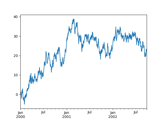
20, Drawing
(1) Getting to know matplotlib
The code is as follows:
ts = pd.Series(np.random.randn(1000), index=pd.date_range('1/1/2000', periods=1000))
ts = ts.cumsum()
ts.plot()
plt.show()
The output results are as follows:
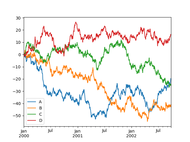
(2) For DataFrame type, plot() can easily draw all columns and their labels
The code is as follows:
ts = pd.Series(np.random.randn(1000), index=pd.date_range('1/1/2000', periods=1000))
df = pd.DataFrame(np.random.randn(1000, 4), index=ts.index, columns=['A', 'B', 'C', 'D'])
df = df.cumsum()
df.plot()
plt.legend(loc='best')
plt.show()
The operation results are as follows:
21, I/O to get data
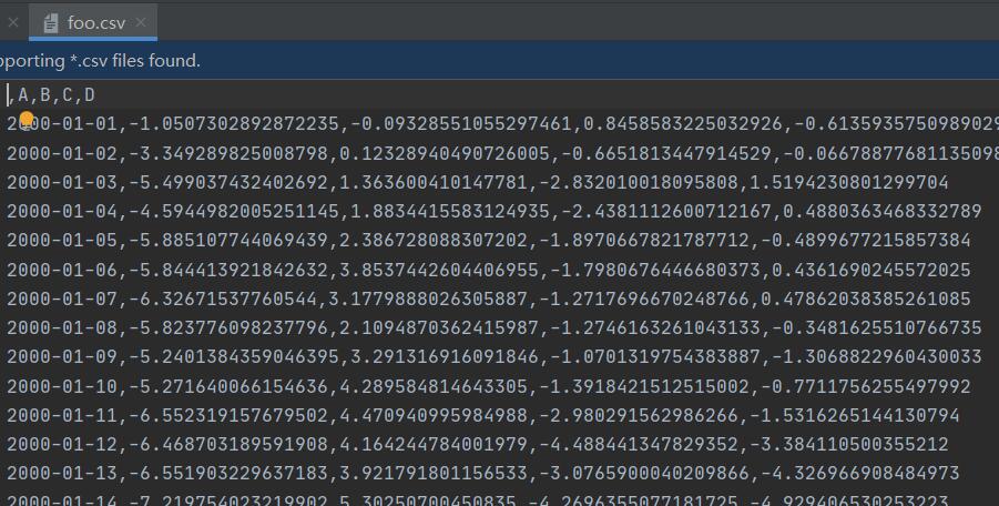
(1) CSV data
Write a csv file:
The code is as follows:
ts = pd.Series(np.random.randn(1000), index=pd.date_range('1/1/2000', periods=1000))
ts = ts.cumsum()
df = pd.DataFrame(np.random.randn(1000, 4), index=ts.index, columns=['A', 'B', 'C', 'D'])
df = df.cumsum()
df.to_csv('data/foo.csv')   # Write a csv file
The generated csv files are as follows:
Read from a csv file:
The code is as follows:
ts = pd.Series(np.random.randn(1000), index=pd.date_range('1/1/2000', periods=1000))
ts = ts.cumsum()
df = pd.DataFrame(np.random.randn(1000, 4), index=ts.index, columns=['A', 'B', 'C', 'D'])
df = df.cumsum()
print(pd.read_csv('foo.csv'))    # Read in a csv file
The output results are as follows:
     Unnamed: 0         A          B          C          D
0    2000-01-01 -1.050730  -0.093286   0.845858  -0.613594
1    2000-01-02 -3.349290   0.123289  -0.665181  -0.066789
2    2000-01-03 -5.499037   1.363600  -2.832010   1.519423
3    2000-01-04 -4.594498   1.883442  -2.438111   0.488036
4    2000-01-05 -5.885108   2.386728  -1.897067  -0.489968
..          ...       ...        ...        ...        ...
995  2002-09-22 -0.637796  12.922019 -24.813859  29.094194
996  2002-09-23 -0.268030  12.872831 -24.495352  28.371192
997  2002-09-24 -0.429714  14.442154 -24.049543  28.734404
998  2002-09-25 -1.868194  12.465456 -22.799273  29.116129
999  2002-09-26 -2.172118  12.427707 -24.062128  28.882752

[1000 rows x 5 columns]

Process finished with exit code 0
(2) HDF5 data
Write an HDF5 Store:
The code is as follows:
ts = pd.Series(np.random.randn(1000), index=pd.date_range('1/1/2000', periods=1000))
ts = ts.cumsum()
df = pd.DataFrame(np.random.randn(1000, 4), index=ts.index, columns=['A', 'B', 'C', 'D'])
df = df.cumsum()
df.to_hdf('foo.h5', 'df')     # write in
The generated files are as follows:

Read from an HDF5 Store:
The code is as follows:
ts = pd.Series(np.random.randn(1000), index=pd.date_range('1/1/2000', periods=1000))
ts = ts.cumsum()
df = pd.DataFrame(np.random.randn(1000, 4), index=ts.index, columns=['A', 'B', 'C', 'D'])
df = df.cumsum()
df.to_hdf('foo.h5', 'df')     # write in
pd.read_hdf('foo.h5', 'df')    # Read in
The output results are as follows:
	               A     	B	       C           	D
2000-01-01	0.544649	-0.048527	-0.069001	0.615770
2000-01-02	-1.375622	-1.001399	-0.461100	-0.314656
2000-01-03	-1.080360	-0.491494	0.058478	-0.263584
2000-01-04	-0.781192	-1.366070	0.713983	0.276506
2000-01-05	-1.726031	-2.226089	1.372384	-1.010998
2000-01-06	-1.029440	-1.116124	3.213516	-1.070904
2000-01-07	-1.132326	0.549860	4.047112	-2.089782
2000-01-08	-1.918885	-0.496898	5.011556	-0.398244
2000-01-09	-2.689141	-0.353073	5.508442	-1.777378
2000-01-10	-0.574410	0.424270	6.674230	-0.836982
2000-01-11	0.968438	0.130614	7.331227	-1.299968
2000-01-12	1.187288	0.447871	8.748361	-2.459602
2000-01-13	1.889565	0.109931	10.110426	-2.873714
2000-01-14	1.549227	0.892440	11.540149	-2.708039
2000-01-15	1.230412	3.760428	11.407844	-3.150406
2000-01-16	0.057691	4.539744	9.338813	-3.744172
2000-01-17	0.004047	4.752471	10.309765	-4.507723
2000-01-18	0.092892	4.859409	9.760544	-3.024875
2000-01-19	1.756680	5.184557	8.991681	-4.547709
2000-01-20	3.133134	5.517767	8.498777	-5.635272
2000-01-21	2.889005	6.491254	8.638766	-6.878007
2000-01-22	2.614277	4.514062	9.359361	-6.409828
2000-01-23	2.004339	5.711879	9.398218	-5.936106
2000-01-24	2.186803	4.852240	8.156034	-6.388658
2000-01-25	3.085273	4.543388	6.914151	-5.814296
2000-01-26	5.203147	4.600532	6.475757	-5.283672
2000-01-27	5.751381	4.626839	8.047942	-3.977368
2000-01-28	5.675581	3.608191	6.809387	-2.812447
2000-01-29	5.401486	2.936898	7.269270	-2.104369
2000-01-30	5.553712	5.005159	8.387554	-2.762008
...	...	...	...	...
2002-08-28	-47.209369	7.254643	8.048536	25.650071
2002-08-29	-46.758124	6.307750	8.852335	25.292648
2002-08-30	-45.177406	5.847630	8.134441	25.595963
2002-08-31	-44.555625	4.738374	9.103920	25.938850
2002-09-01	-44.594843	4.847349	7.607951	26.767106
2002-09-02	-45.468864	3.460726	7.441725	27.277645
2002-09-03	-48.126574	4.654244	5.223401	27.618957
2002-09-04	-47.503283	4.500056	6.162534	28.210921
2002-09-05	-47.770849	3.965948	6.850322	28.129603
2002-09-06	-47.103058	3.908913	7.081636	29.309787
2002-09-07	-48.252013	4.328563	8.561459	29.842983
2002-09-08	-48.335899	2.360573	8.865642	30.591404
2002-09-09	-46.875850	2.844337	7.152740	31.220225
2002-09-10	-47.242826	2.538062	6.462508	30.843580
2002-09-11	-47.881749	3.812996	6.520225	32.369875
2002-09-12	-46.864357	4.713924	6.569562	32.144355
2002-09-13	-45.546403	2.981736	8.046595	33.097245
2002-09-14	-44.470824	4.739932	7.934668	32.488292
2002-09-15	-44.206498	3.851915	6.901387	31.004478
2002-09-16	-45.192152	2.235635	7.017709	30.362812
2002-09-17	-45.775304	3.109701	5.925081	30.872055
2002-09-18	-45.652522	4.743547	4.843658	29.608422
2002-09-19	-47.494023	4.842967	3.590295	29.586813
2002-09-20	-47.098042	5.926378	4.235130	29.989704
2002-09-21	-48.317910	4.805615	5.094592	30.270280
2002-09-22	-48.432906	5.759228	4.651891	30.817247
2002-09-23	-47.112905	6.014631	4.202600	29.703626
2002-09-24	-46.085425	6.468472	3.649689	29.517390
2002-09-25	-44.384026	5.569878	3.598782	29.982023
2002-09-26	-42.653887	5.947389	4.319416	31.901769
1000 rows × 4 columns
(3) Excel data
Write to an Excel file:
ts = pd.Series(np.random.randn(1000), index=pd.date_range('1/1/2000', periods=1000))
ts = ts.cumsum()
df = pd.DataFrame(np.random.randn(1000, 4), index=ts.index, columns=['A', 'B', 'C', 'D'])
df = df.cumsum()

df.to_excel('foo.xlsx', sheet_name='Sheet1')    # Write excel
Note: import dependent libraries and module s.
The generated excel file is as follows:
Read from an Excel file:
ts = pd.Series(np.random.randn(1000), index=pd.date_range('1/1/2000', periods=1000))
ts = ts.cumsum()
df = pd.DataFrame(np.random.randn(1000, 4), index=ts.index, columns=['A', 'B', 'C', 'D'])
df = df.cumsum()


print(pd.read_excel('foo.xlsx', 'Sheet1', index_col=None, na_values=['NA']))
The operation results are as follows:
    Unnamed: 0          A          B          C          D
0   2000-01-01   1.161650   0.711842   0.355790  -0.465520
1   2000-01-02   0.303399   0.266687   0.029220  -0.304709
2   2000-01-03   0.525579   1.834383  -1.003671   0.202279
3   2000-01-04   0.733337   3.045663  -2.245458   2.095680
4   2000-01-05   0.107569   3.380991  -4.067166   0.423934
..         ...        ...        ...        ...        ...
995 2002-09-22 -16.517889 -14.676465  18.354474  72.024858
996 2002-09-23 -16.714840 -13.742384  17.133618  72.441209
997 2002-09-24 -15.751055 -15.707861  17.496880  73.232321
998 2002-09-25 -14.977084 -16.827697  17.091075  72.890022
999 2002-09-26 -15.173852 -17.319843  16.150347  71.989576

[1000 rows x 5 columns]

Process finished with exit code 0
be careful:
When I write code, I make an error: pandas can't be opened Xlsx file, xlrd biffh. XLRDError: Excel xlsx file; not supported
Reason: the reason is that xlrd has been updated to version 2.0.1 recently and only supports xls file. So pandas read_ Excel ('xxx.xlsx ') will report an error. Legacy xlrd can be installed.
Solution: under windows10, enter the project folder D:\dream\venv\Scripts (my path is this) and use cmd to enter this directory for installation.
pip install xlrd==1.2.0
Alternatively, openpyxl can be used instead of xlrd xlsx file:
df=pandas.read_excel('data.xlsx',engine='openpyxl')
Postscript
Finally, I recommend you to use anaconda when learning python. It integrates ipython, Jupiter notebook, etc. it is convenient to write code. When I write this question, I use python. Some libraries have problems, but using Jupiter notebook works normally. Well, that's all for today and continue to study tomorrow.