How to run

• Installation dependency

pip install keras
pip install pygame
pip install scikit-image
pip install h5py

The author uses theano training. The trained model file can only be called by using theano as the backend of Keras in the configuration file ~ / Keras/keras. Confirm / modify the backend to theano in JSON (if tensorflow [another optional backend of Keras] is not installed), and the configuration file style is shown in the supplement to the convolution neural network section below.
To use theano, we also need to install OpenBLAS . Directly download the source code and unzip it, cd it into the directory, and then

sudo apt-get install gfortran
make FC=gfortran  
sudo make PREFIX=/usr/local install  

• Download the source code and run it

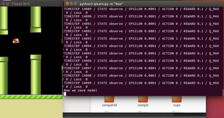
git clone https://github.com/yanpanlau/Keras-FlappyBird.git
cd Keras-FlappyBird
python qlearn.py -m "Run"

Game / wrapped in my download directory\_ flappy\_ bird. Py file, line 144, fpslock There is a problem with the indentation at the tick (FPS) statement. Delete the existing indentation and type 8 spaces. If there is no problem, don't worry.

• vmware virtual machine Ubuntu 16 04 + Python 3 + only use CPU+theano to run:

• If you want to retrain the neural network, delete the model H5 file and then run the command qlearn py -m "Train".

Source code analysis

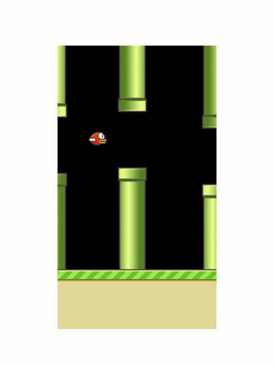
• Game input and return images

import wrapped_flappy_bird as game
x_t1_colored, r_t, terminal = game_state.frame_step(a_t)

Directly use the flappybird python version of the interface.
Enter a\_t ((1,0) means no jump, (0,1) means jump).
The return value is the next frame image x\_t1\_colored and reward (+ 0.1 for survival, + 1 for passing through the pipeline, and - 1 for death). The reward is controlled at [- 1, + 1] to improve stability. terminal is a Boolean value indicating whether the game is over.
Reward function in game/wrapped_flappy_bird.py
def frame_step(self, input_actions) method.

Why directly input the game image for processing? I didn't turn the corner at first, In fact, the image contains all the information (sound information is only an aid in most games and does not affect the game), and people also accept the input image information when playing the game, and then decide to output the corresponding operation instructions. This is actually simulating the human feedback process, describing this process as a nonlinear function, which we will use convolution neural network to express, generally convolution real The image feature is extracted, and the neural network realizes the conversion from feature to operation instruction.

• Image preprocessing

essential factor:

1.  Convert picture to gray scale
2.  Crop picture size to 80 x80 pixel
3.  Four frames are stacked each time and fed into the neural network together. It is equivalent to entering one at a time'Four channels'Image of.  
    (Why stack 4 frames together? This is a method to enable the model to infer the speed information of the bird.)

x_t1 = skimage.color.rgb2gray(x_t1_colored)
x_t1 = skimage.transform.resize(x_t1,(80,80))
x_t1 = skimage.exposure.rescale_intensity(x_t1, out_range=(0, 255)) # adjust brightness
#
x_t1 = x_t1.reshape(1, 1, x_t1.shape[0], x_t1.shape[1])
s_t1 = np.append(x_t1, s_t[:, :3, :, :], axis=1)
# axis=1 means adding on the second dimension

x\_t1 is a (1x1x80x80) single frame, s\_t1 is the superposition of 4 frames in the shape of (1x4x80x80). The input is designed as (1x4x80x80) instead of (4x8xx80x80) for Keras consideration.

supplement

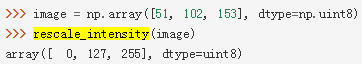
rescale\_intensity

• Convolutional neural network
  Now, the preprocessed image is input into the neural network.

def buildmodel():
    print("Start modeling")
    model = Sequential()
    model.add(Convolution2D(32, 8, 8, subsample=(4,4),init=lambda shape, name: normal(shape, scale=0.01, name=name), border_mode='same', dim_ordering='th', input_shape=(img_channels,img_rows,img_cols)))
    model.add(Activation('relu'))
    model.add(Convolution2D(64, 4, 4, subsample=(2,2),init=lambda shape, name: normal(shape, scale=0.01, name=name), border_mode='same', dim_ordering='th'))
    model.add(Activation('relu'))
    model.add(Convolution2D(64, 3, 3, subsample=(1,1),init=lambda shape, name: normal(shape, scale=0.01, name=name), border_mode='same', dim_ordering='th'))
    model.add(Activation('relu'))
    model.add(Flatten())
    model.add(Dense(512, init=lambda shape, name: normal(shape, scale=0.01, name=name)))
    model.add(Activation('relu'))
    model.add(Dense(2,init=lambda shape, name: normal(shape, scale=0.01, name=name)))
   
    adam = Adam(lr=1e-6)
    model.compile(loss='mse',optimizer=adam)
    print("Modeling complete")
    return model

Convolution2D(
nb\_filter, # number of filters
nb\_row, # filter rows
nb\_col, # number of columns of the filter
init='glorot\_uniform ', # layer weights initialization function
activation='linear ', # by default, the activation function is linear, that is, a(x) = x
weights=None,
border\_mode='valid',
\#The default is' valid '(zero is not filled, generally)
\#Or 'same' (auto zeroing so that the output size is the same as the input size when the filter window step is 1,
\#I.e. output size = input size / stride)
subsample=(1, 1), # represents the left and down filter window movement steps
dim\_ Ordering ='default ', #' default 'or' tf 'or' th '
W\_regularizer=None,
b\_regularizer=None,
activity\_regularizer=None,
W\_constraint=None,
b\_constraint=None,
bias=True
\#Uncommented generally use the default value
)

The function is the convolution function of the filter window of two-dimensional input.
When using it as the first layer of the model, you need to provide`input_shape`Keyword, such as 128 x128 RGB 3 Channel image, then`input_shape=(3, 128, 128)`. `dim_ordering`The default value for is`~/.keras/keras.json`In the file, if none can be created (generally run once) keras Yes), the format is

{
"image\_dim\_ordering": "tf",
"epsilon": 1e-07,
"floatx": "float32",
"backend": "tensorflow"
}

according to`image_dim_ordering`and`backend`Select use`theano`Namely`th`perhaps`tensorflow`Namely`tf`. 

- The exact structure is as follows:
The input is 4 x80x80 Image matrix.
The first convolution layer has 32 convolution cores (filters), and the size of each convolution core is 8 x8，x Shaft and y The strides of the axes are all 4, zero filled, and one is used ReLU Activate the function.
The second convolution layer has 64 convolution cores (filters), and the size of each convolution core is 4 x4，x Shaft and y The strides of the axes are 2, zero filled, and one is used ReLU Activate the function.
The third convolution layer has 64 convolution cores (filters), and the size of each convolution core is 3 x3，x Shaft and y The strides of the axes are all 1, zero filled, and one is used ReLU Activate the function.
Then flatten them into a one-dimensional input hidden layer. The hidden layer has 512 neural units, all connected to the output of the third layer convolution layer and used ReLU Activate the function.
The final output layer is a fully connected linear layer, which corresponds to the output action Q List of values. Generally speaking, index 0 means doing nothing; In this game, index 1 represents a jump. Compare the two Q Select the larger value as the next operation.
> For relevant knowledge points, please see:
[Convolutional neural network CNN Basic concept notes](http://www.jianshu.com/p/606a33ba04ff)
[CS231n Convolutional Neural Networks](http://cs231n.github.io/convolutional-networks/)
Output calculation formula of each layer:(W-F+2P)/S+1. 
W:Enter size; S:stride; F:Convolution kernel size; P:Make up zero.
In the setup of this application, the output calculation can be simplified to W/S. 

![Structure diagram](http://upload-images.jianshu.io/upload_images/2422746-ca7a2f32e0f2e692.png?imageMogr2/auto-orient/strip%7CimageView2/2/w/1240)
> Supplement: see[Draw the structure diagram of convolution neural network](http://www.jianshu.com/p/56a05b5e4f20)

- Tips 
keras It makes the construction of convolutional neural network very simple. But there are some things to pay attention to.
A. It is important to choose a good initialization method, which is selected hereσ=0.01 Normal distribution of.(`lambad x,y : f(x,y)`Is an anonymous function)
`init=lambda shape, name: normal(shape, scale=0.01, name=name)`
B. The order of dimensions is important. use Theano It's 4 x80x80，Tensorflow If yes, the input is 80 x80x4. adopt Convolution2D Functional**dim_ordering**Parameter settings are used here theano. 
C. An adaptive optimization algorithm called Adam is used this time. The learning rate is**1-e6**. 
D. On gradient descent optimization algorithm[An overview of gradient descent optimization algorithms](http://sebastianruder.com/optimizing-gradient-descent/). 
E. `Convolution2D`Parameters in function`border_mode`It should also be noted that the zero filling operation is selected here, so that the pixels at the edge of the image are also filtered and all image information is transformed.

- DQN
 The following is the application Q-learning Algorithm to train the neural network.
stay Q-learning The most important thing is Q The function: **Q(s, a)**Represents when we are in a state s implement a Maximum discount reward for action. **Q(s, a)**Give you a question about s Status selection a How good the action is.
Q Functions are like the secrets of playing a game when you need to decide on the state s Select the next action a still b When, just lift it up Q Value action is OK.
**Maximum discount Award**Both reflected in s Make action in state a Get status s'Immediate feedback reward (survival)+0.1，Through pipe+1)，Also reflected in the state s'The best possible reward for continuing the game (no matter what input) - is actually s'For all actions**In the maximum discount reward**The largest of (i.e`max[ Q(s', a) | All possible actions a]`)，But the second reward should be multiplied by a discount coefficient, because it is a future reward. If you want to discount, you have to give a discount.
actually Q Function is a function with theoretical assumptions. We can see from the above expression Q The function can be expressed as a recursive form, and we can obtain it through iteration, which coincides with the training process of neural network.
And we want to use convolutional neural network to realize it Q Function, actually(Q,a) = f(s)Function, which returns all possible inputs in a state and the corresponding Q A list of binary pairs composed of values, but the input actions are represented by different indexes. In this way, we save the state of giant many s Analysis, judgment and complex programming, as long as it is initialized in some way Q Value table, and then according to Q The weight of the neural network is adjusted by the value table training, and then updated according to the prediction of the trained neural network Q Value table, so repeated iterations to approximate Q Function.

        # Take a small batch of samples for training
        minibatch = random.sample(D, BATCH)
        # inputs and targets together form a Q-value table
        inputs = np.zeros((BATCH, s_t.shape[1], s_t.shape[2], s_t.shape[3]))   #32, 80, 80, 4
        targets = np.zeros((inputs.shape[0], ACTIONS))                         #32, 2

        # Start experience playback
        for i in range(0, len(minibatch)):
            # The following sequence number corresponds to the storage order of D to take out all the information,
            # D.append((s_t, action_index, r_t, s_t1, terminal))
            state_t = minibatch[i][0]    # current state
            action_t = minibatch[i][1]   # Input action
            reward_t = minibatch[i][2]   # Return reward
            state_t1 = minibatch[i][3]   # Return to next status
            terminal = minibatch[i][4]   # Flag returned whether to terminate

            inputs[i:i + 1] = state_t    # Save the current state, i.e. s in Q(s,a)

            # Get a list of predicted Q values indexed by input action x
            targets[i] = model.predict(state_t)  
            # Get the list of Q values predicted in the next state with the input action x as the index
            Q_sa = model.predict(state_t1)

            if terminal:  # If the game terminates after the action is executed, the Q value of (s) the action (a) in this state is equivalent to the reward
                targets[i, action_t] = reward_t
            else:         # Otherwise, the Q value of the action (a) in this state (s) is equivalent to the immediate reward after the action is executed and the best expected reward in the next state multiplied by a discount rate
                targets[i, action_t] = reward_t + GAMMA * np.max(Q_sa)

        # The neural network is trained with the generated Q-value table, and the current error is returned at the same time
        loss += model.train_on_batch(inputs, targets)

- Experience replay
  In the above code, there is an experience replay( Experience Replay). In fact, nonlinear functions such as neural networks are used to Q The value approximation is very unstable. The most important trick to solve this problem is to replay the experience. All staged scenes in the game are placed in the playback memory**D**Yes. (used here) python of deque Structure to store). When training neural networks, from**D**The stability of the system will be greatly improved by extracting scenarios in small batch rather than using the latest ones.
- Exploration and development
 This is another problem of reinforcement learning: continue to explore new resources or focus on developing existing resources. That is, how to choose and allocate time between exploiting existing known good decisions and continuing to explore new and possibly better behaviors. In real life, we often encounter this kind of problem: choose a tried restaurant or try a new one - it may be better or it may not eat at all. In reinforcement learning, in order to maximize future benefits, it must strike a balance between the two. A popular solution is calledϵ(epsilon)Greedy method.ϵIs a variable between 0 and 1, according to which time it can get to explore a random new action.

        if random.random() <= epsilon:
            print("----------Random Action----------")
            action_index = random.randrange(ACTIONS)
            a_t[action_index] = 1
        else:
            q = model.predict(s_t)       #Input the combination of four images to predict the results
            max_Q = np.argmax(q)
            action_index = max_Q
            a_t[max_Q] = 1

### Work that can be improved
1.  current DQN Based on a lot of experience, whether it is possible to replace it or delete it.
2. How to determine the best convolution neural network.
3. Training is slow. How to speed it up or make it converge faster.
4. What does convolutional neural network learn and whether its learning results are transferable.

### Other resources
- [Demystifying Deep Reinforcement Learning](https://www.nervanasys.com/demystifying-deep-reinforcement-learning/)
- [Uncover the secrets of intensive learning (Chinese translation of the above English article)](http://chuansong.me/n/335655551424)
- [Keras plays catch, a single file Reinforcement Learning example](http://edersantana.github.io/articles/keras_rl/)
- [Human-level control through deep reinforcement learning](http://www.nature.com/nature/journal/v518/n7540/full/nature14236.html)
- [Above(Human-level)of ppt Lecture notes](http://ir.hit.edu.cn/~jguo/docs/notes/dqn-atari.pdf)
- [Configuring Theano For High Performance Deep Learning](http://www.johnwittenauer.net/configuring-theano-for-high-performance-deep-learning/)

### code annotation

!/usr/bin/env python

from future import print\_function

import argparse
import skimage as skimage
from skimage import transform, color, exposure
from skimage.transform import rotate
from skimage.viewer import ImageViewer
import sys
sys.path.append("game/")
import wrapped\_flappy\_bird as game
import random
import numpy as np
from collections import deque

import json
from keras import initializations
from keras.initializations import normal, identity
from keras.models import model\_from\_json
from keras.models import Sequential
from keras.layers.core import Dense, Dropout, Activation, Flatten
from keras.layers.convolutional import Convolution2D, MaxPooling2D
from keras.optimizers import SGD , Adam

GAME = 'bird' # game name
CONFIG = 'nothreshold'
ACTIONS = 2 # effective actions: immobile + jump = 2
GAMMA = 0.99 # discount coefficient. Future rewards are converted into a coefficient to be multiplied by current rewards
OBSERVATION = 3200. # How many steps are observed before training
EXPLORE = 3000000. # Total steps of epsilon attenuation
FINAL\_ Epsilon = minimum value of 0.0001 # epsilon
INITIAL\_ Epsilon = the initial value of 0.1 # epsilon, and epsilon decreases gradually
REPLAY\_MEMORY = 50000 # remembered scenarios (all information from state s to state s')
BATCH = 32 # selected number of small batch training samples

One input action per frame

FRAME\_PER\_ACTION = 1

Image size after preprocessing

img\_rows , img\_cols = 80, 80

Stack 4 gray-scale images each time, equivalent to 4 channels

img\_channels = 4

Constructing neural network model

def buildmodel():
print("Now we build the model")
\#The following notes are provided in the text
model = Sequential()
model.add(Convolution2D(32, 8, 8, subsample=(4,4),init=lambda shape, name: normal(shape, scale=0.01, name=name), border\_mode='same',input\_shape=(img\_channels,img\_rows,img\_cols)))
model.add(Activation('relu'))
model.add(Convolution2D(64, 4, 4, subsample=(2,2),init=lambda shape, name: normal(shape, scale=0.01, name=name), border\_mode='same'))
model.add(Activation('relu'))
model.add(Convolution2D(64, 3, 3, subsample=(1,1),init=lambda shape, name: normal(shape, scale=0.01, name=name), border\_mode='same'))
model.add(Activation('relu'))
model.add(Flatten())
model.add(Dense(512, init=lambda shape, name: normal(shape, scale=0.01, name=name)))
model.add(Activation('relu'))
model.add(Dense(2,init=lambda shape, name: normal(shape, scale=0.01, name=name)))

adam = Adam(lr=1e-6)
model.compile(loss='mse',optimizer=adam) # The loss function is used as the mean square error, and the optimizer is Adam.
print("We finish building the model")
return model

def trainNetwork(model,args):
\#Get a game simulator
game\_state = game.GameState()

# The observed playback memory D before saving
D = deque()

# Do nothing to get the first state, and then preprocess the picture in 80x80x4 format
do_nothing = np.zeros(ACTIONS)
do_nothing[0] = 1  # do_nothing is array([1,0])
x_t, r_0, terminal = game_state.frame_step(do_nothing)

x_t = skimage.color.rgb2gray(x_t)
x_t = skimage.transform.resize(x_t,(80,80))
x_t = skimage.exposure.rescale_intensity(x_t,out_range=(0,255))
# During initialization, all 4 stacked graphs are the same as the initial one
s_t = np.stack((x_t, x_t, x_t, x_t), axis=0)  # s_t is the stack of four figures

# In order to use in Keras, we need to adjust the array shape and add a dimension in the header
s_t = s_t.reshape(1, s_t.shape[0], s_t.shape[1], s_t.shape[2])

if args['mode'] == 'Run':
    OBSERVE = 999999999    # We always observe, not train
    epsilon = FINAL_EPSILON
    print ("Now we load weight")
    model.load_weights("model.h5")
    adam = Adam(lr=1e-6)
    model.compile(loss='mse',optimizer=adam)
    print ("Weight load successfully")    
else:                      # Otherwise, we start training after observing for a period of time
    OBSERVE = OBSERVATION
    epsilon = INITIAL_EPSILON

t = 0 # t is the total number of frames
while (True):
    # Value of each cycle reinitialization
    loss = 0
    Q_sa = 0
    action_index = 0
    r_t = 0
    a_t = np.zeros([ACTIONS])
    # Select behavior through epsilon greedy algorithm
    if t % FRAME_PER_ACTION == 0:
        if random.random() <= epsilon:
            print("----------Random Action----------")
            action_index = random.randrange(ACTIONS) # Pick an action at random
            a_t[action_index] = 1        # Generate corresponding normalized action input parameters
        else:
            q = model.predict(s_t)       # Enter the current state to get the predicted Q value
            max_Q = np.argmax(q)         # Returns the index of the largest value in the array
            # numpy.argmax(a, axis=None, out=None)
            # Returns the indices of the maximum values along an axis.
            action_index = max_Q         # Index 0 means doing nothing, and index 1 means jumping
            a_t[max_Q] = 1               # Generate corresponding normalized action input parameters

    # After training and before epsilon is less than a certain value, we gradually reduce epsilon
    if epsilon > FINAL_EPSILON and t > OBSERVE:
        epsilon -= (INITIAL_EPSILON - FINAL_EPSILON) / EXPLORE

    # Perform the selected action and observe the next status and reward returned
    x_t1_colored, r_t, terminal = game_state.frame_step(a_t)
    # The image is processed into gray scale, and the size and brightness are adjusted
    x_t1 = skimage.color.rgb2gray(x_t1_colored)
    x_t1 = skimage.transform.resize(x_t1,(80,80))
    x_t1 = skimage.exposure.rescale_intensity(x_t1, out_range=(0, 255))
    # Adjust the shape of the image array to increase the first two dimensions to four dimensions
    x_t1 = x_t1.reshape(1, 1, x_t1.shape[0], x_t1.shape[1])
    # Will s_ The first three frames of T are added after the new frame, and the index of the new frame is 0 to form the last four frames of image
    s_t1 = np.append(x_t1, s_t[:, :3, :, :], axis=1)


    # The storage state is transferred to the playback memory
    D.append((s_t, action_index, r_t, s_t1, terminal))
    if len(D) > REPLAY_MEMORY:
        D.popleft()

    # If the observation is complete, then
    if t > OBSERVE:
        # Take a small batch of samples for training
        minibatch = random.sample(D, BATCH)
        # inputs and targets together form a Q-value table
        inputs = np.zeros((BATCH, s_t.shape[1], s_t.shape[2], s_t.shape[3]))   #32, 80, 80, 4
        targets = np.zeros((inputs.shape[0], ACTIONS))                         #32, 2

        # Start experience playback
        for i in range(0, len(minibatch)):
            # The following sequence number corresponds to the storage order of D to take out all the information,
            # D.append((s_t, action_index, r_t, s_t1, terminal))
            state_t = minibatch[i][0]    # current state
            action_t = minibatch[i][1]   # Input action
            reward_t = minibatch[i][2]   # Return reward
            state_t1 = minibatch[i][3]   # Return to next status
            terminal = minibatch[i][4]   # Flag returned whether to terminate

            inputs[i:i + 1] = state_t    # Save the current state, i.e. s in Q(s,a)

            # Get a list of predicted Q values indexed by input action x
            targets[i] = model.predict(state_t)  
            # Get the list of Q values predicted in the next state with the input action x as the index
            Q_sa = model.predict(state_t1)

            if terminal:  # If the game terminates after the action is executed, the Q value of (s) the action (a) in this state is equivalent to the reward
                targets[i, action_t] = reward_t
            else:         # Otherwise, the Q value of the action (a) in this state (s) is equivalent to the immediate reward after the action is executed and the best expected reward in the next state multiplied by a discount rate
                targets[i, action_t] = reward_t + GAMMA * np.max(Q_sa)

        # The neural network is trained with the generated Q-value table, and the current error is returned at the same time
        loss += model.train_on_batch(inputs, targets)

    s_t = s_t1 # The next state becomes the current state
    t = t + 1  # Total frames + 1

    # Store the current training model every 100 iterations
    if t % 100 == 0:
        print("Now we save model")
        model.save_weights("model.h5", overwrite=True)
        with open("model.json", "w") as outfile:
            json.dump(model.to_json(), outfile)

    # Output information
    state = ""
    if t <= OBSERVE:
        state = "observe"
    elif t > OBSERVE and t <= OBSERVE + EXPLORE:
        state = "explore"
    else:
        state = "train"

    print("TIMESTEP", t, "/ STATE", state, \
        "/ EPSILON", epsilon, "/ ACTION", action_index, "/ REWARD", r_t, \
        "/ Q_MAX " , np.max(Q_sa), "/ Loss ", loss)

print("Episode finished!")
print("************************")

def playGame(args):
model = buildmodel() # build the model first
trainNetwork(model,args) # start training

def main():
parser = argparse.ArgumentParser(description='Description of your program')
parser.add\_argument('-m','--mode', help='Train / Run', required=True) # accepts the parameter mode
args = vars(parser.parse\_args()) # args is the dictionary and 'mode' is the key
playGame(args) # start the game

if name == "main":
main() # when executing this script, start with the main function