brief introduction

Simply put: in the distance space, if most of the k nearest neighbors of a sample belong to a category, the sample also belongs to this category.
API official website link
api

class sklearn.neighbors.KNeighborsClassifier(n_neighbors=5, *, weights='uniform', algorithm='auto', leaf_size=30, p=2, metric='minkowski', metric_params=None, n_jobs=None)

Parameter Description:
n_neighbors – select several neighbors to reference. Default = 5

algorithm: {'auto'，'ball_tree'，'kd_tree'，'brute'}

• The default parameter of fast k-nearest neighbor search algorithm is auto, which can be understood as that the algorithm determines the appropriate search algorithm by itself. In addition, users can also specify their own search algorithm ball_tree,kd_ Search by tree and brute methods,
  • Brute is brute force search, that is, linear scanning. When the training set is large, the calculation is very time-consuming.
  • kd_tree is a tree data structure that constructs a KD tree to store data for rapid retrieval. KD tree is also a binary tree in the data structure. For the tree constructed by median segmentation, each node is a super rectangle, and the time efficiency is high when the dimension is less than 20.
  • ball tree is invented to overcome the high latitude failure of kd tree. Its construction process is to divide the sample space with centroid C and radius r, and each node is a hypersphere.

leaf_size: optional parameter (30 by default). This is the size of the construction tree. Generally, the default value can be selected. Too much will affect the speed.

n_jobs: the default value is 1. Selecting - 1 will reduce the proportion of CPU, but the running speed will also slow down, and all core s will run.

P: distance parameter (2 by default)
P is derived from the "minkovsky distance"
Only when the KNN algorithm considers the distance weight super parameter (weights), will it consider whether to input the distance parameter (P)

K value selection

K value is too small:
Vulnerable to outliers
Over fitting
The model is too complex
k value is too large:
The problem of sample equilibrium
Under fitting
The model is too simple

kd-tree

According to KNN, every time we need to predict a point, we need to calculate the distance from each point in the training data set to this point, and then select the nearest k points for voting. When the data set is large, the computational cost is very high. For the data set with N samples and D features, the algorithm complexity is O (DN^2).

kd tree: in order to avoid recalculating the distance every time, the algorithm saves the distance information in A tree. In this way, the distance information is queried from the tree before calculation to avoid recalculation as much as possible. The basic principle is that if A and B are far away and B and C are close, then A and C are far away. With this information, you can skip distant points at the right time.

In this way, the complexity of the optimized algorithm can be reduced to O (DNlog (N)). Interested readers can refer to the paper: Bentley, J.L., Communications of the ACM (1975).

In 1989, another algorithm called Ball Tree further optimized the performance based on kd Tree. Interested readers can search Five balltree construction algorithms for detailed algorithm information.

(1) Select the one dimension of the vector to divide;

(2) How to divide data;

The simple solution to the first problem can be to randomly select a certain dimension or select it in order, but a better method should be to divide it in the dimension where the data are scattered (the degree of dispersion can be measured according to variance). A good partition method can make the constructed tree more balanced, and the median can be selected for partition each time. In this way, problem 2 has also been solved.

case analysis
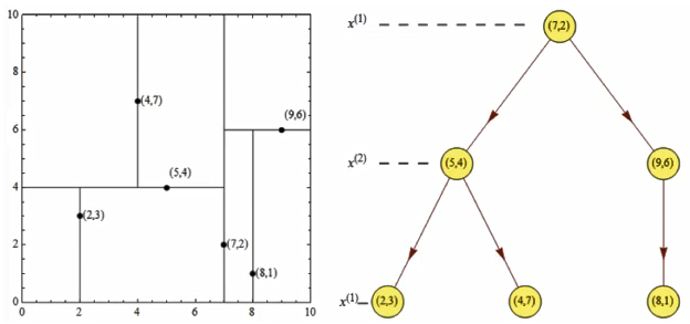
Given a two-dimensional spatial data set: T={(2,3),(5,4),(9,6),(4,7),(8,1),(7,2)}, a balanced kd tree is constructed.
for the first time:
x-axis – 2, 5, 9, 4, 8, 7 – > 2, 4, 5, 7, 8, 9
y-axis – 3, 4, 6, 7, 1, 2 – > 1, 2, 3, 4, 6, 7
The x-axis data is scattered. First select the x-axis and find the middle point. It is found that it is (7, 2)
The second time:
Left: (2, 3), (4, 7), (5, 4) – > 3, 4, 7
Right: (8, 1), (9, 6) – > 1, 6
Select from the y-axis. The selection points on the left are (5, 4), the selection points on the right (9, 6) – there are only two numbers on the right, and any one in the middle can be selected
third time:
Select from the x axis

Find the closest point (2.1, 3.1) in the above dataset

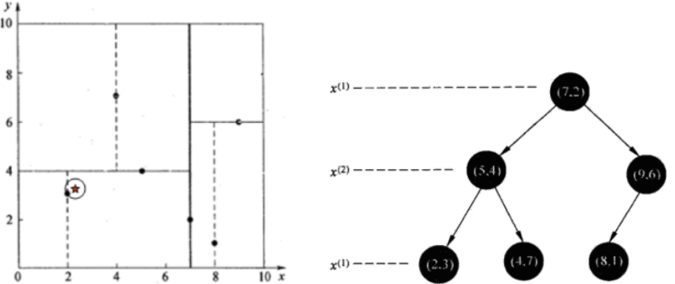
According to the above traversal method of comparing the size of the x-axis for the first time, the size of the y-axis for the second time, and the x-axis for the third time.
Test arrival (5,4) at point (7,2), test arrival (2,3) at point (5,4), and then search_ The nodes in path are < (7,2), (5,4), (2,3) >, from search_ Take (2,3) from path as the current best node nearest, and dist is 0.141;

Then trace back to (5,4), draw a circle with (2.1,3.1) as the center and dist=0.141 as the radius, and it does not intersect with hyperplane y=4, as shown in the figure above, so it is not necessary to jump to the right subspace of node (5,4) to search, because there can be no closer sample points in the right subspace.

So we go back to (7,2). Similarly, we draw a circle with (2.1,3.1) as the center and dist=0.141 as the radius, which does not intersect with hyperplane x=7, so we don't have to jump to the right subspace of node (7,2) to search.

So far, search_ If path is empty, end the whole search and return nearest(2,3) as the nearest neighbor of (2.1,3.1), with the nearest distance of 0.141.

Also, find the closest point (2,4.5) in the above dataset

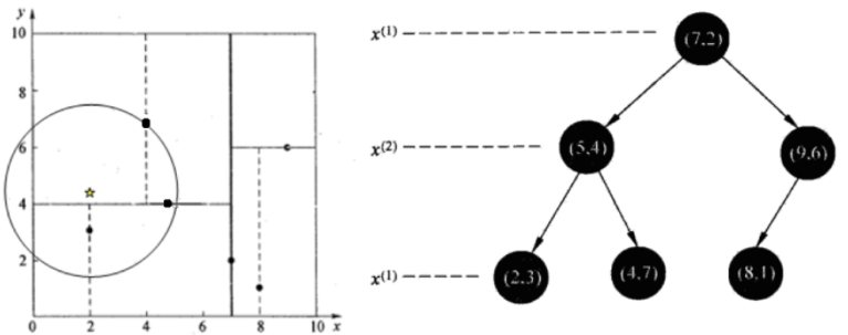
Test arrival at (5,4) at (7,2), test arrival at (4,7) at (5,4) [search in this field first], and then search_ The nodes in path are < (7,2), (5,4), (4,7) >, from search_ Take (4,7) from path as the current best node nearest, and dist is 3.202;

Then trace back to (5,4), draw a circle with (2,4.5) as the center and dist=3.202 as the radius, intersecting with hyperplane y=4, so you need to jump to the left subspace of (5,4) to search. So add (2,3) to search_path, now search_ The nodes in path are < (7,2), (2,3) >; In addition, the distance between (5,4) and (2,4.5) is 3.04 < dist=3.202, so (5,4) is assigned to nearest, and dist=3.04.

Backtracking to (2,3), (2,3) is the leaf node. Directly judge whether (2,3) is closer to (2,4.5). The calculated distance is 1.5, so the nearest is updated to (2,3) and dist is updated to (1.5)

Go back to (7,2). Similarly, draw a circle with (2,4.5) as the center and dist=1.5 as the radius, which does not intersect with hyperplane x=7, so you don't have to jump to the right subspace of node (7,2) to search.

So far, search_ If path is empty, end the whole search and return nearest(2,3) as the nearest neighbor of (2,4.5), with the nearest distance of 1.5.

Advantages and disadvantages

advantage:
1. Simple and effective (it can solve multi classification problems and regression problems naturally)
2. Retraining cost
3. Suitable for class domain cross samples
4. Suitable for automatic classification of large samples
Disadvantages:
1. Inert learning
2. The category score is not standardized
3. The output interpretability is not strong
4. Not good at unbalanced samples
Sample imbalance: the proportion of each category of data collected is seriously unbalanced
5. Large amount of calculation

k-nearest neighbor algorithm is the simplest and most effective algorithm for classifying data. When using the algorithm, we must have training sample data close to the actual data. k-nearest neighbor algorithm must save all data sets. If the training data set is large, we must use a lot of storage space. In addition, because the distance value must be calculated for each data in the dataset, it may be very time-consuming in actual use.

Another defect of k-nearest neighbor algorithm is that it can not give any data infrastructure information, so we can not know the characteristics of average instance samples and typical instance samples.

Example

Iris species prediction / film classification

#Iris species prediction
from sklearn.datasets import load_iris
from sklearn.model_selection import train_test_split
from  sklearn.preprocessing import StandardScaler
from sklearn.neighbors import KNeighborsClassifier

# 1. Get data set
iris = load_iris()

# 2. Basic data processing
# x_train,x_test,y_train,y_test is the training set eigenvalue, test set eigenvalue, training set target value and test set target value
x_train, x_test, y_train, y_test = train_test_split(iris.data, iris.target, test_size=0.2, random_state=22)

# 3. Feature Engineering: Standardization
transfer = StandardScaler()
x_train = transfer.fit_transform(x_train)
x_test = transfer.transform(x_test)

# 4. Machine learning (model training)
#4.1 instantiate a converter
estimator = KNeighborsClassifier(n_neighbors=9)
#4.2 model training
estimator.fit(x_train, y_train)

# 5. Model evaluation
# Method 1: compare the real value with the predicted value
y_predict = estimator.predict(x_test)
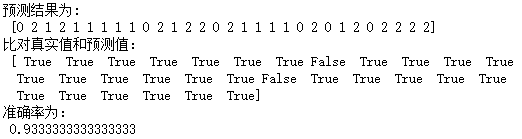
print("The prediction result is:\n", y_predict)
print("Compare the real value with the predicted value:\n", y_predict == y_test)
# Method 2: calculate the accuracy directly
score = estimator.score(x_test,y_test)
print("The accuracy is:\n", score)

# Movie data classification
from sklearn import neighbors  # Import KNN classification module
import numpy as np
import pandas as pd
import matplotlib.pyplot as plt
plt.rcParams['font.sans-serif'] = ['KaiTi']

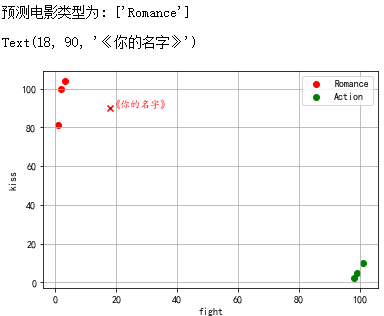
data = pd.DataFrame({'name':['Beijing meets Seattle','like you','Zootopia','Warwolf 2','King Li','dare-to-die corps'],
                  'fight':[3,2,1,101,99,98],
                  'kiss':[104,100,81,10,5,2],
                  'type':['Romance','Romance','Romance','Action','Action','Action']})

knn = neighbors.KNeighborsClassifier()   # Get knn classifier
knn.fit(data[['fight','kiss']], data['type'])
print('The predicted movie type is:', knn.predict([[18, 90]]))
# Load data and build KNN classification model
# Predict unknown data

plt.scatter(data[data['type'] == 'Romance']['fight'],data[data['type'] == 'Romance']['kiss'],color = 'r',marker = 'o',label = 'Romance')
plt.scatter(data[data['type'] == 'Action']['fight'],data[data['type'] == 'Action']['kiss'],color = 'g',marker = 'o',label = 'Action')
plt.grid()
plt.legend()
plt.scatter(18,90,color = 'r',marker = 'x',label = 'Romance')
plt.ylabel('kiss')
plt.xlabel('fight')
plt.text(18,90,'<Your name',color = 'r')
# Draw a chart