Modeling and kinematics simulation of three-axis manipulator

  before starting the design of specific mechanical structure and driving structure, it is necessary to carry out kinematic simulation on the manipulator to obtain its forward kinematics solution, inverse kinematics solution and workspace.

    in the primary school that just ended, we disassembled and simulated the kinematics of a real six axis manipulator, and then finished the project report. I thought that this simulation could be slightly changed in the summer code, but - after all, I paid by mistake.

Personal understanding of each simulation project

   before starting, I need to talk about several parts of simulation from the perspective of application: solution of forward and inverse solutions, workspace analysis and trajectory planning. First of all, the general goal of manipulator design should be clear, that is, to design a device that can reach the specified pose according to the specified scheme.
The two requirements of specifying scheme and pointing pose in the above understanding put forward requirements for the process of design and trajectory planning, and these requirements should also be considered in kinematic modeling and simulation.

• Kinematics forward and inverse solution: the solution of the forward and inverse solution will be used in two parts, namely, the initial determination of relevant parameters of DH array list and the solution of trajectory planning. The process of determining DH parameters is to change the parameters again and again, verify the positive and negative solutions, and judge whether the current parameters can meet the requirements of reaching the specified pose; In the process of trajectory planning, the use of forward and inverse solutions is mainly inverse solutions, that is, to solve the joint angles of the end point and the middle point to achieve different trajectory planning effects.
• Trajectory planning: the process of trajectory planning is the process of realizing the specified motion scheme. Its role is self-evident, so it is not repeated.
• Workspace: I don't understand the analysis of workspace. During the previous study, I thought he just drew the boundary between reachable and unreachable machines to divide the work forbidden area to protect workers. Until I began to adjust the arm length by solving the forward and inverse solutions.
  I found that you can filter through the workspace

Difficulties in analysis of three-axis manipulator (underactuated)

   three dimensional space has six degrees of freedom, three degrees of freedom of movement and three degrees of freedom of rotation. A manipulator with less than six degrees of freedom is called an underactuated manipulator (I didn't check, but it should be)
  if the robot has fewer degrees of freedom, it can not specify any position and attitude at will, but can only move to the desired position and the attitude limited by fewer joints. That is, there are few arbitrary reachable points in the workspace of underactuated robots, especially for 3-DOF robots, there is only one pose at many working points, that is, there is only one pose at one position.
   the inverse solution of the RTB toolbox in MATLAB needs to input the T matrix of the target point (including position and attitude at the same time), but we can't do it without constraints on attitude in our actual needs, so the inverse solution program of RTB is not feasible. In order to find an appropriate inverse solution, I have made the following attempts:

Change the source code of inverse solution in RTB

The analysis in primary school should have been to analyze the code for solving the inverse solution, but for various reasons, it was mainly lazy and did not proceed. Finally, I went around and returned to the origin. In short, I started with the source code:

• In the first paragraph, the mask variable is a matrix with one row and six columns, which can be defined according to the actual degree of freedom of the manipulator. The first few numbers are 1 and the rest are 0 before solving;

   assert(numel(opt.mask) == 6, 'RTB:ikine:badarg', 'Mask matrix should have 6 elements');
   assert(n >= numel(find(opt.mask)), 'RTB:ikine:badarg', 'Number of robot DOF must be >= the number of 1s in the mask matrix');
   W = diag(opt.mask);

• The second code defines how to compare the current value with the target value to approach the target value when solving. The core code is the tr2delta function in the first line. This function is also a part of RTB toolbox, which is used to solve the differential motion matrix from the current value to the target value, and measure the error by calculating the norm of the matrix. End the calculation when it is less than the defined end error opt.tol;

  e = tr2delta(robot.fkine(q), T);        
  % are we there yet
      if norm(W*e) < opt.tol
      break;

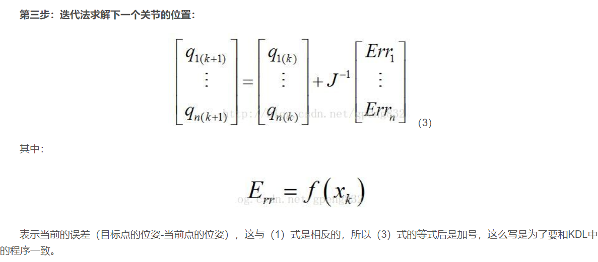
• The third code is the process of iterative calculation, which is the real core. The code adopts the Jacobian matrix iteration method mentioned in the textbook, which has been explained by some people. See here for details:
  [robotics] robot open source project KDL source code learning: (2) numerical solution of robot by Newton Raphson iterative method

while true
    % calculation error
    Tq = robot.fkine(q');
    e(1:3) = transl(T - Tq);
    Rq = t2r(Tq);
    [th,n] = tr2angvec(Rq'*t2r(T));
    e(4:6) = th*n;
    
    J = jacob0(robot, q);   % Calculate Jacobi
    % The joint change is calculated according to the end error
    if opt.pinv  % Jacobian pseudo inverse method
        dq = opt.alpha * pinv( J(m,:) ) * e(m);
    else         % Jacobian transposition
        dq = J(m,:)' * e(m);
        dq = opt.alpha * dq;
    end

    % Update joint values
    q = q + dq';

    % Judge whether the error is less than the allowable error tolerance
    nm = norm(e(m));
    if nm <= opt.tol
        break
    end

  after analyzing the code, start to change the code. I can only say that I know a little about the iterative part of Jacobian matrix, so the changed part can be in the error comparison link. The last thing we want is the position of the space point, and there is no requirement for its attitude. Therefore, we want to minimize the impact of attitude on the results, so we make the following modifications:

   aaa=robot.fkine(q);
    e=T-aaa;
    e=e(:,4);
    e(4:6,:)=0;
    %e = tr2delta(robot.fkine(q), T);

  the error is changed to the norm of the position difference between the current point and the final point, that is, the error is determined only by the position, but after the experiment, it is found that the result is not much different from the source code. In fact, I'm very desperate to change here. After all, it took a long time to check the data and read the code, but the project still has to continue. I can only comfort myself: at least I understand the code
In addition, there is a parameter list for solving the inverse solution of RTB, which is shared here

% set defaultparameters for solution Default parameter settings
opt.ilimit = 500; %Default number of iterations
opt.rlimit = 100; %Maximum number of consecutive rejections
opt.slimit = 100; %Maximum number of attempts
opt.tol = 1e-10; %Default iteration error
opt.lambda = 0.1; %Default step size
opt.lambdamin = 0; %Default step size minimum
opt.search = false; %Default off search initial value
opt.quiet = false; %Keep quiet and reduce output
opt.verbose = false; %Output details
opt.mask = [1 1 1 1 1 1]; %Default six degrees of freedom

Find analytical solution

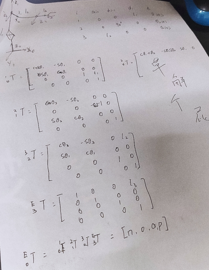
   the analytical solution expression of the three degree of freedom robot is relatively simple, which can be obtained directly from geometric knowledge without matrix transformation, as shown in the following figure:

  however, with my poor mathematical knowledge, I can't solve this system of ternary nonlinear equations by listing a few pages of calculus. Therefore, this method is stillborn.

Numerical solution

  although the previous method did not let us find the analytical solution, we finally obtained the nonlinear equations with three joint variables. Matlab also has a set of relevant algorithms for numerically solving nonlinear equations, so in the attitude of violent solution, I read some relevant posts in the MATLAB community. Finally, I found a tutorial on solving the analytical solution of the two degree of freedom manipulator by quasi Newton method, which is linked as follows:
MATLAB two degree of freedom analytical solution
Referring to its idea and code, the code for solving the analytical solution by numerical method can be achieved by bringing in the above three degrees of freedom analytical solution equation, including the following two parts:

Numerical solution:

//Numerical solution
function [x,fval,exitflag]=Robot_Inverse_Solution(a,b,c)
x=a;
y=b;
z=c;
l1=0.18;
l2=0.15;
l3=0.03;
options=optimset('display','off','MaxFunEvals',1000000,'TolFun',1e-3);
[x,fval,exitflag]=fsolve('threeJoint',[0 0.1 0.1],options,l1,l2,l3,x,y,z);

end

Definition of nonlinear equation:

//Definition of nonlinear equation
function F=threeJoint(theta,l1,l2,l3,x,y,z)

theta1=theta(1);
theta2=theta(2);
theta3=theta(3);

% F1=x-l2*cos(theta2)*cos(theta1)-l3*cos(theta2+theta3)*cos(theta1);
% F2=y-l2*cos(theta2)*sin(theta1)-l3*cos(theta2+theta3)*sin(theta1);
% F3=z-l1-l2*sin(theta2)*-l3*sin(theta2+theta3);

F=[F1,F2,F3];
end

   this method is sensitive to the initial value, so the interest interval of the input joint variable theta has a great impact on the accuracy of the solution results. In most cases, we can not give a very appropriate estimate, so this method is not suitable for practical application in theory.
This is also reflected in the specific solution process. I tried a group of better solutions:

theta=[0，pi/3，0]；

Nevertheless, the result is still not ideal, which is still a failed attempt.

Workspace filtering

  in the face of successive failures, I decided to give up the inverse solution for the time being and conduct workspace analysis first. Monte Carlo method is used to analyze the workspace. Each joint variable of the manipulator can produce N pseudo-random values, that is, the value of the joint variable is substituted into the forward kinematics equation of the manipulator in the order from small to large, the position direction of the end effector in the reference coordinate is obtained, and the obtained position vector of the manipulator is drawn as the workspace of the manipulator.
  during the analysis, I suddenly thought that since the Monte Carlo method has generated 10000 or even 100000 work points, can we find the appropriate work points through screening?

    q1_rand = q1_s*angle + unifrnd(0,1,[num,1])*(q1_end - q1_s)*angle;
    q2_rand = q2_s*angle + unifrnd(0,1,[num,1])*(q2_end - q2_s)*angle;
    q3_rand = q3_s*angle + unifrnd(0,1,[num,1])*(q3_end - q3_s)*angle;
    q4_rand = rand(num,1)*0;
    q = [q1_rand q2_rand q3_rand q4_rand];
    fk=modrobot.fkine(q).t;%Forward kinematics simulation function index=zeros(1,5000)
		for i=1:5000
   			 t=fk(1,i);
   			 t=transl(t)	%from SE3 The matrix is changed to a matrix that can be operated directly
   			 %%Specific competition process
   			 if (abs(t(1,2)-0.01)<0.001)&(abs(t(1,1)-0.01)<0.001)
   			 end
        	 if(abs(t(1,1)-0.01)<0.001&(abs(t(1,1)-0.01)<0.001)
        	 end
             if(abs(t(1,3)-0.01)<0.001&(abs(t(1,3)-0.01)<0.001)
               index(1,i)=1;
   	         end
end

  the program can realize this function and return the index of a set of solutions that meet the conditions. In other words, the workspace can provide safe area division and can also be used to screen appropriate inverse kinematics solutions. However, this method has a large amount of calculation and is only suitable for the initial determination of robot configuration, which is not practical in trajectory planning,

Practical analytical solution

   I have successfully completed the initial task, but the writing of blog has dragged the front for a long time, from more than August to today. That is, today, in teacher Zhang Aijun's class, Professor Saeed B.Niku's robotics brought me new hope - the analytical solution is solvable!

   I wanted to solve the inverse solution by hand, but the result is as shown in the figure. On the way to solve the inverse solution, I died on the way to solve the positive solution. At this time, let's open the MATLAB in our hands:

syms th1 th2 th3  l1 l2 l3 ;
syms nx ny nz ax ay az ox oy oz px py pz;
TT=[nx,ox,ax,px;
    ny,oy,ay,py;
    nz,oz,az,pz;
    0,0,0,1];


%Coordinate system winding Z Transformation matrix of axis rotation Tz
Tz1=[ cos(th1) sin(th1) 0 0;
    -sin(th1) cos(th1) 0 0;
    0         0        1 0;
    0 0 0 1]; 

Tz2=[ cos(th2) sin(th2) 0 0;
    -sin(th2) cos(th2) 0 0;
    0         0        1 0;
    0 0 0 1]; 

Tz3=[ cos(th3) sin(th3) 0 0;
    -sin(th3) cos(th3) 0 0;
    0         0        1 0;
    0 0 0 1]; 
%Positive solution
T1=trotx(0)*transl([0 0 0])*Tz1*transl([0 0 l1]);
T2=trotx(90)*transl([0 0 0])*Tz2*transl([0 0 0]);
T3=trotx(0)*transl([l2 0 0])*Tz3*transl([0 0 0]);
T4=transl([l3 0 0]);

%Paul Inverse transformation
T=T1*T2*T3*T4
t1=T_ink(T1)*TT
t11= T2*T3*T4
    

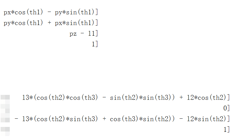
The figure shows the p vectors on both sides after the first Paul inverse transformation. After being brought into p2, the result is just the same as that in the book

   in fact, the difficulties of the three degree of freedom manipulator mentioned above do not constitute here, because the inverse solution can be solved easily by using Paul inverse transformation method. Even here, there is a general idea for the four axis five week underactuated manipulator, that is, in addition to paying attention to the p vector on both sides, you can pay more attention to the rotation around the axis in one direction, but this is all later.

summary

Very simple idea, very naive attempt, and tried for a lot of time; The idea of building a manipulator has done the first step of simulation, debugging the top-level MoveIt code, writing the PWM drive of DC motor and serial communication... After writing this blog, it is assembly and debugging, which is another large number of work.
It's impossible to guarantee the postgraduate entrance examination. It's too early to take the postgraduate entrance examination. Anyway, it's idle. Do something interesting and meaningful.

It's time for junior to harvest