catalogue
2.1 advantages and disadvantages of the algorithm
3. Distance formula in the algorithm
4.5 separate training set and test set
4.6 calculation of Euclidean distance
5. Implementation of scikit learn algorithm
5.1 re realization of the above:
5.2 another implementation method
1. Basic definitions
k-nearest neighbor algorithm is a relatively simple machine learning algorithm. It uses the method of measuring the distance between different eigenvalues for classification. Its idea is very simple: if most of the samples of multiple nearest neighbors (most similar) in the feature space belong to a category, the sample also belongs to this category. The first letter k can be lowercase, indicating the number of externally defined nearest neighbors.
In short, let the machine itself according to the distance of each point, and the close ones are classified as one kind.
2. Algorithm principle
The core idea of knn algorithm is the category of unlabeled samples, which is decided by the nearest k neighbors.
Specifically, suppose we have a labeled data set. At this time, there is an unmarked data sample. Our task is to predict the category of this data sample. The principle of knn is to calculate the distance between the sample to be labeled and each sample in the data set, and take the nearest K samples. The category of the sample to be marked is generated by the voting of the k nearest samples.
Suppose X_test is the sample to be marked, X_train is a marked data set, and the pseudo code of algorithm principle is as follows:
- Traverse x_ For all samples in the train, calculate the relationship between each sample and X_test and save the Distance in the Distance array.
- Sort the Distance array, take the nearest k points and record them as X_knn.
- In X_ Count the number of each category in KNN, that is, class0 is in X_ There are several samples in KNN, and class1 is in X_ There are several samples in KNN.
- The category of samples to be marked is in X_ The category with the largest number of samples in KNN.
2.1 advantages and disadvantages of the algorithm
- Advantages: high accuracy, high tolerance to outliers and noise.
- Disadvantages: large amount of calculation and large demand for memory.
2.2 algorithm parameters
The algorithm parameter is k, and the parameter selection needs to be determined according to the data.
- The larger the k value is, the greater the deviation of the model is, and the less sensitive it is to noise data. When the k value is large, it may cause under fitting;
- The smaller the k value, the greater the variance of the model. When the k value is too small, it will cause over fitting.
2.3 variants
There are some variants of knn algorithm, one of which can increase the weight of neighbors. By default, the same weight is used when calculating the distance. In fact, you can specify different distance weights for different neighbors. For example, the closer the distance, the higher the weight. This can be achieved by specifying the weights parameter of the algorithm.
Another variant is to replace the nearest k points with points within a certain radius. When the data sampling is uneven, it can have better performance. In scikit learn, the RadiusNeighborsClassifier class implements this algorithm variant.
3. Distance formula in the algorithm
Unlike our linear regression, we have no formula to deduce here. The core of KNN classification algorithm is to calculate the distance, and then classify according to the distance.
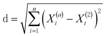
In the two-dimensional Cartesian coordinate system, I believe junior high school students should be familiar with this. He has a more common name, rectangular coordinate system. Among them, Euclidean distance is commonly used to calculate the distance between two points. Point A(2,3) and point B(5,6), then the distance of AB is
This is the Euclidean distance. However, there are some differences from what we often encounter. Euclidean distance can calculate multidimensional data, that is, matrix. This can help us solve many problems, so the formula becomes
4. Case realization
We used the knn algorithm and its variants to predict the diabetes of Pina Indians. The dataset can be downloaded from below.
Link: LAN Zuoyun
4.1 import related libraries
# Import related modules
import numpy as np
from collections import Counter
import matplotlib.pyplot as plt
from sklearn.utils import shuffle
import pandas as pd
4.2 reading data
#Read data
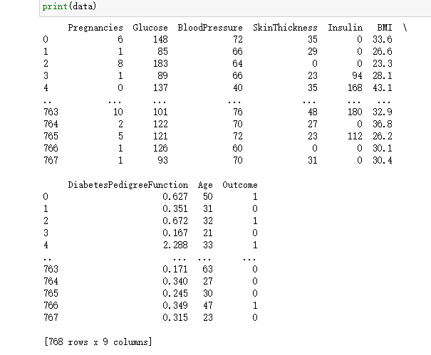
data=pd.read_excel('D:\desktop\knn.xlsx')
print(data)return:
4.3 read variable name
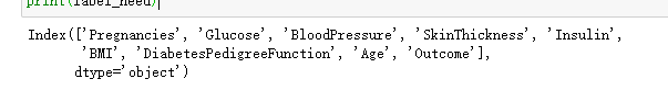
label_need=data.keys()
print(label_need)
return:
4.4 define X,Y data
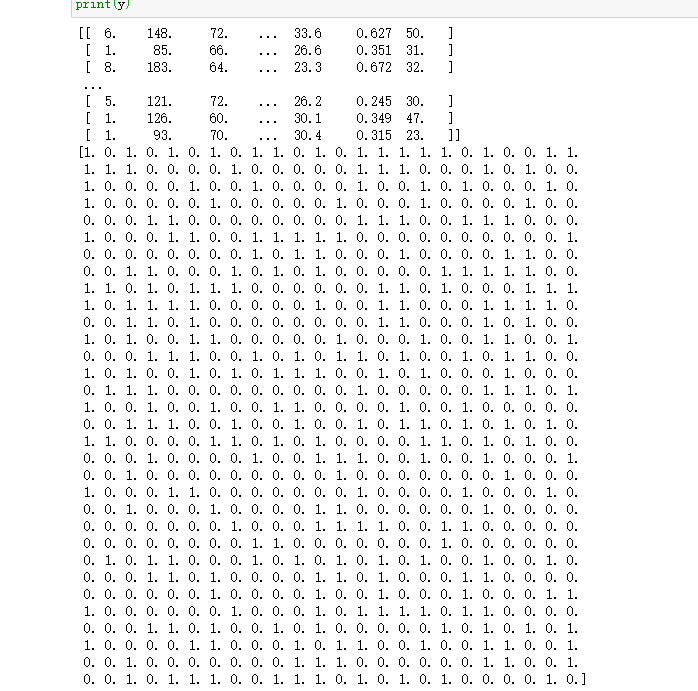
X = data[label_need].values[:,0:8]
y = data[label_need].values[:,8]
print(X)
print(y)
return:
4.5 separate training set and test set
from sklearn.model_selection import train_test_split
X_train, X_test, y_train,y_test = train_test_split(X, y, test_size=0.2)
# Print training set and test set size
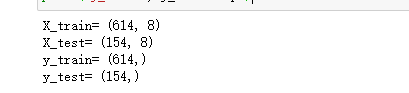
print('X_train=', X_train.shape)
print('X_test=', X_test.shape)
print('y_train=', y_train.shape)
print('y_test=', y_test.shape)return:
4.6 calculation of Euclidean distance
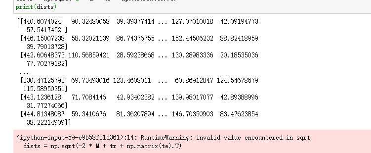
# Sample size of test case
num_test = X.shape[0]
# Training instance sample size
num_train = X_train.shape[0]
# Euclidean distance initialization based on training and testing dimensions
dists = np.zeros((num_test, num_train))
# Matrix point multiplication of test samples and training samples
M = np.dot(X, X_train.T)
# Test sample matrix square
te = np.square(X).sum(axis=1)
# Square of training sample matrix
tr = np.square(X_train).sum(axis=1)
# Calculate Euclidean distance
dists = np.sqrt(-2 * M + tr + np.matrix(te).T)
print(dists)
return:
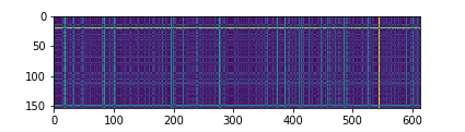
4.7 # visual distance matrix
dists = compute_distances(X_test, X_train)
plt.imshow(dists, interpolation='none')
plt.show()
return:
4.8 forecast samples
# Test sample size
num_test = dists.shape[0]
# Initialize test set prediction results
y_pred = np.zeros(num_test)
# ergodic
for i in range(num_test):
# Initialize nearest neighbor list
closest_y = []
# Take the index after sorting according to the Euclidean distance matrix, and take the value according to the sorted index with the training set label
# Final flattening list
# Note NP Usage of argsort function
labels = y_train[np.argsort(dists[i, :])].flatten()
# Take the nearest k values
closest_y = labels[0:k]
# Count the latest k values
# Here, notice the usage of Counter in the collections module
c = Counter(closest_y)
# Take the category with the highest count
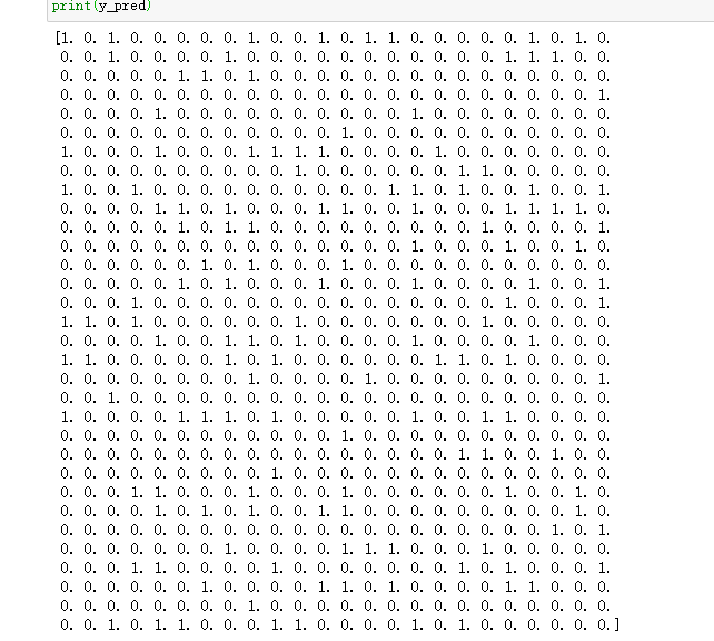
y_pred[i] = c.most_common(1)[0][0]
print(y_pred)return:
4.9 check the accuracy
Check the number of actual and predicted matches:
# Find examples of correct predictions
num_correct = np.sum(y_test_pred == y_test)
print(num_correct)
return:
Calculation accuracy:
# Calculation accuracy
accuracy = float(num_correct) / X_test.shape[0]
print('Got %d/%d correct=>accuracy:%f'% (num_correct, X_test.shape[0], accuracy))
return:

4.10 cross validation
# Fold cross validation
num_folds = 5
# Candidate k value
k_choices = [1, 3, 5, 8, 10, 12, 15, 20, 50, 100]
X_train_folds = []
y_train_folds = []
# Training data division
X_train_folds = np.array_split(X_train, num_folds)
# Training label Division
y_train_folds = np.array_split(y_train, num_folds)
k_to_accuracies = {}
# Traverse all candidate k values
for k in k_choices:
    # Five fold traversal
    for fold in range(num_folds):
        # Separate a verification set for the incoming training set as the test set
        validation_X_test = X_train_folds[fold]
        validation_y_test = y_train_folds[fold]
        temp_X_train = np.concatenate(X_train_folds[:fold] + X_train_folds[fold + 1:])
        temp_y_train = np.concatenate(y_train_folds[:fold] + y_train_folds[fold + 1:])
        # Calculate distance
        temp_dists = compute_distances(validation_X_test, temp_X_train)
        temp_y_test_pred = predict_labels(temp_y_train, temp_dists, k=k)
        temp_y_test_pred = temp_y_test_pred.reshape((-1, 1))
        # View classification accuracy
        num_correct = np.sum(temp_y_test_pred == validation_y_test)
        num_test = validation_X_test.shape[0]
        accuracy = float(num_correct) / num_test
        k_to_accuracies[k] = k_to_accuracies.get(k,[]) + [accuracy]
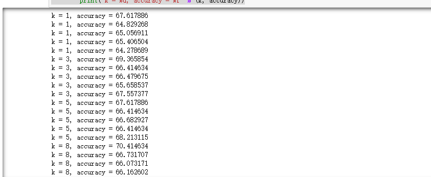
Print the classification accuracy under different k values and different discounts:
# Print the classification accuracy under different k values and different discounts
for k in sorted(k_to_accuracies):
      for accuracy in k_to_accuracies[k]:
        print('k = %d, accuracy = %f' % (k, accuracy))
return:
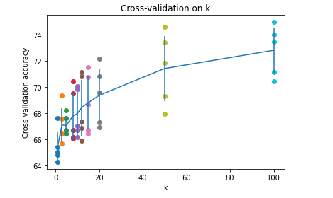
Visualization of classification accuracy under different k values and different discounts:
for k in k_choices:
    # Take out the classification accuracy of the k-th k-value
    accuracies = k_to_accuracies[k]
    # Plot scatter plots with different accuracy of k value
    plt.scatter([k] * len(accuracies), accuracies)
# Calculate the mean value of accuracy and sort
accuracies_mean = np.array([np.mean(v) for k,v in sorted(k_to_accuracies.items())])
# Calculate the standard deviation of accuracy and sort
accuracies_std = np.array([np.std(v) for k,v in sorted(k_to_accuracies.items())])
# Draw error bar chart with confidence interval
plt.errorbar(k_choices, accuracies_mean, yerr=accuracies_std)
# Drawing title
plt.title('Cross-validation on k')
# x-axis label
plt.xlabel('k')
# y-axis label
plt.ylabel('Cross-validation accuracy')
plt.show()
return:
5. Implementation of scikit learn algorithm
5.1 re realization of the above:
# Import kneigborsclassifier module
from sklearn.neighbors import KNeighborsClassifier
# Create k nearest neighbor instance
neigh = KNeighborsClassifier(n_neighbors=10)
# k-nearest neighbor model fitting
neigh.fit(X_train, y_train)
# k-nearest neighbor model prediction
y_pred = neigh.predict(X_test)
# # Reconstruction of prediction result array
# y_pred = y_pred.reshape((-1, 1))
# Count the number of correct predictions
num_correct = np.sum(y_pred == y_test)
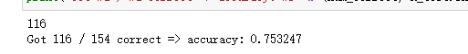
print(num_correct)
# Calculation accuracy
accuracy = float(num_correct) / X_test.shape[0]
print('Got %d / %d correct => accuracy: %f' % (num_correct, X_test.shape[0], accuracy))return:
5.2 another implementation method
5.2.1 loading data
import pandas as pd
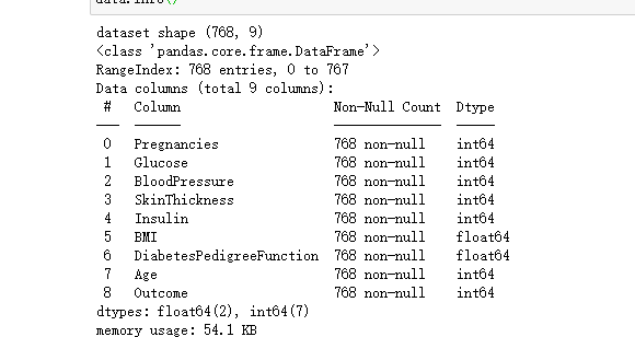
data = pd.read_csv('D:\desktop\knn.csv')
print('dataset shape {}'.format(data.shape))
data.info()return:
5.2.2 separate training set and test set
X = data.iloc[:, 0:8]
Y = data.iloc[:, 8]
print('shape of X {}, shape of Y {}'.format(X.shape, Y.shape))

from sklearn.model_selection import train_test_split
X_train, X_test, Y_train,Y_test = train_test_split(X, Y, test_size=0.2)
return:

5.2.3 model comparison
The common knn algorithm, weighted knn algorithm and specified radius knn algorithm are used to calculate the score of the data set
from sklearn.neighbors import KNeighborsClassifier, RadiusNeighborsClassifier

# Build three models
models = []
models.append(('KNN', KNeighborsClassifier(n_neighbors=2)))
models.append(('KNN with weights', KNeighborsClassifier(n_neighbors=2, weights='distance')))
models.append(('Radius Neighbors', RadiusNeighborsClassifier(n_neighbors=2, radius=500.0)))

# Train three models respectively and calculate the score
results = []
for name, model in models:
    model.fit(X_train, Y_train)
    results.append((name, model.score(X_test, Y_test)))
for i in range(len(results)):
    print('name: {}; score: {}'.format(results[i][0], results[i][1]))
return:
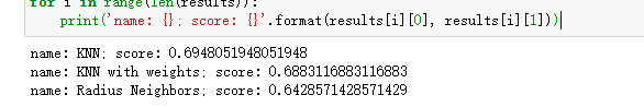
For the weight algorithm, we choose the closer the distance, the higher the weight. The radius of the radius neighbors classifier model is 500 It can be seen from the output that the ordinary knn algorithm is still the best.
Here comes the question. Is this judgment accurate? The answer is: inaccurate.
Because our training set and test set are randomly assigned, different combinations of training samples and test samples may lead to differences in the accuracy of the calculated algorithm.
So how to solve it?
We can randomly assign the training set and cross validation set for many times, and then calculate the average value of the model score.
Scikit learn provides KFold and cross_val_score() function to handle this problem.
from sklearn.model_selection import KFold
from sklearn.model_selection import cross_val_score

results = []
for name, model in models:
    kfold = KFold(n_splits=10)
    cv_result = cross_val_score(model, X, Y, cv=kfold)
    results.append((name, cv_result))

for i in range(len(results)):
    print('name: {}; cross_val_score: {}'.format(results[i][0], results[i][1].mean()))
return:
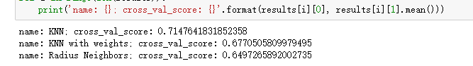
For the above code, we divide the data set into 10 parts through KFold, of which 1 will be used as the cross validation set to calculate the model accuracy, and the remaining 9 will be used as the training set. cross_ val_ The score () function calculates the model scores obtained from the combination of 10 different training sets and cross validation sets, and finally calculates the average value. It seems that the performance of ordinary knn algorithm is better.
5.2.4} model training and analysis
According to the conclusion obtained from the above model comparison, we then use the ordinary knn algorithm model to train the data set, and check the fitting of the training samples and the prediction accuracy of the test samples:
knn = KNeighborsClassifier(n_neighbors=2)
knn.fit(X_train, Y_train)
train_score = knn.score(X_train, Y_train)
test_score = knn.score(X_test, Y_test)
print('train score: {}; test score : {}'.format(train_score, test_score))
return:

From here, we can see two problems.
- The fitting of training samples is poor, and the score is only more than 0.84, indicating that the algorithm model is too simple to fit the training samples well.
- The accuracy of the model is not good, and the prediction accuracy is about 0.66.
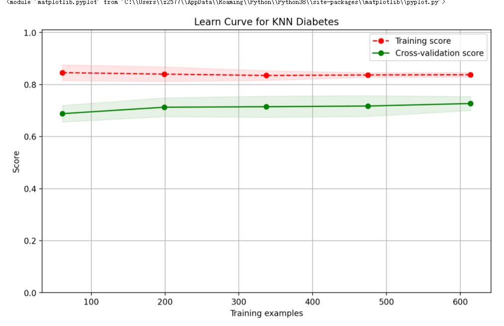
Let's draw a curve and have a look.
Let's first define the drawing function. The code is as follows:
from sklearn.model_selection import learning_curve
import numpy as np

def plot_learning_curve(plt, estimator, title, X, y, ylim=None, cv=None,
                        n_jobs=1, train_sizes=np.linspace(.1, 1.0, 5)):
    """
    Generate a simple plot of the test and training learning curve.

    Parameters
    ----------
    estimator : object type that implements the "fit" and "predict" methods
        An object of that type which is cloned for each validation.

    title : string
        Title for the chart.

    X : array-like, shape (n_samples, n_features)
        Training vector, where n_samples is the number of samples and
        n_features is the number of features.

    y : array-like, shape (n_samples) or (n_samples, n_features), optional
        Target relative to X for classification or regression;
        None for unsupervised learning.

    ylim : tuple, shape (ymin, ymax), optional
        Defines minimum and maximum yvalues plotted.

    cv : int, cross-validation generator or an iterable, optional
        Determines the cross-validation splitting strategy.
        Possible inputs for cv are:
          - None, to use the default 3-fold cross-validation,
          - integer, to specify the number of folds.
          - An object to be used as a cross-validation generator.
          - An iterable yielding train/test splits.

        For integer/None inputs, if ``y`` is binary or multiclass,
        :class:`StratifiedKFold` used. If the estimator is not a classifier
        or if ``y`` is neither binary nor multiclass, :class:`KFold` is used.

        Refer :ref:`User Guide <cross_validation>` for the various
        cross-validators that can be used here.

    n_jobs : integer, optional
        Number of jobs to run in parallel (default 1).
    """
    plt.title(title)
    if ylim is not None:
        plt.ylim(*ylim)
    plt.xlabel("Training examples")
    plt.ylabel("Score")
    train_sizes, train_scores, test_scores = learning_curve(
        estimator, X, y, cv=cv, n_jobs=n_jobs, train_sizes=train_sizes)
    train_scores_mean = np.mean(train_scores, axis=1)
    train_scores_std = np.std(train_scores, axis=1)
    test_scores_mean = np.mean(test_scores, axis=1)
    test_scores_std = np.std(test_scores, axis=1)
    plt.grid()

    plt.fill_between(train_sizes, train_scores_mean - train_scores_std,
                     train_scores_mean + train_scores_std, alpha=0.1,
                     color="r")
    plt.fill_between(train_sizes, test_scores_mean - test_scores_std,
                     test_scores_mean + test_scores_std, alpha=0.1, color="g")
    plt.plot(train_sizes, train_scores_mean, 'o--', color="r",
             label="Training score")
    plt.plot(train_sizes, test_scores_mean, 'o-', color="g",
             label="Cross-validation score")

    plt.legend(loc="best")
    return plt
Then we call this function and draw the following figure:
from sklearn.model_selection import ShuffleSplit

knn = KNeighborsClassifier(n_neighbors=2)
cv = ShuffleSplit(n_splits=10, test_size=0.2, random_state=0)
plt.figure(figsize=(10,6), dpi=200)
plot_learning_curve(plt, knn, 'Learn Curve for KNN Diabetes', X, Y, ylim=(0.0, 1.01), cv=cv)
return: