1 basic knowledge of image
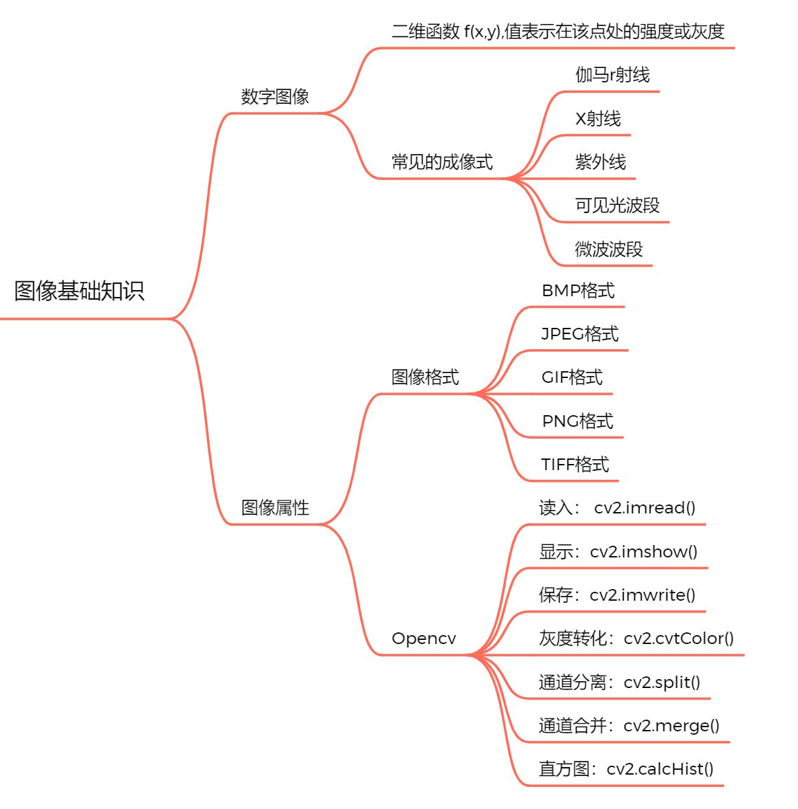
1.1 digital image
A two-dimensional image can be represented by a matrix or array. We can understand it as a binary function f ( x , y ) f(x,y) f(x,y), where x x x and y y y is the space coordinate, f f f represents the value at this coordinate, that is, the intensity or gray level of the image at this point.
Common imaging methods include:
| name | wavelength | nature | application |
|---|---|---|---|
| γ \gamma γ radial | < 1 0 − 10 <10^{-10} <10−10 | It is emitted from the nucleus, with strong penetration ability and great destructive power to organisms | Brain physiological signal EGG |
| χ \chi χ radial | ( 10 − 0.01 ) × 1 0 − 9 (10-0.01)×10^{-9} (10−0.01)×10−9 | Different parts have different absorption rates | CT |
| ultraviolet rays | ( 380 − 10 ) × 1 0 − 9 (380-10)×10^{-9} (380−10)×10−9 | Chemical effect | Biomedical field |
| visible light | ( 7.8 − 3.8 ) × 1 0 − 7 (7.8-3.8)×10^{-7} (7.8−3.8)×10−7 | Light shines on objects and is reflected into people's eyes | |
| infrared | ( 1000 − 0.78 ) × 1 0 − 6 (1000-0.78)×10^{-6} (1000−0.78)×10−6 | All objects in nature can radiate infrared rays | Infrared image; Infrared temperature measurement |
| microwave | 0.1 c m − 1 m 0.1cm-1m 0.1cm−1m | radiation | Radar; Communication system; Microwave image |
| radio frequency | 0.1 c m − 3000 m 0.1cm-3000m 0.1cm−3000m | Television; radio broadcast; medical imaging |
1.2 image attributes
Image format
BMP: uncompressed, large file;
JPEG: lossy compression, widely used on the Internet;
GIF: it can be animation and supports transparent background, but the color gamut is not too wide;
PNG: the compression ratio is higher than GIF, supporting transparent images, and the transparency can be adjusted through Alpha channel;
TIFF: the image format is complex and the storage information is rich, which is used for printing;
The size of the image is in pixels. The gray pixel value ranges from 0 to 255. 0 represents black and 255 represents white.
Image resolution: the number of pixels per unit length.
Number of channels: the bit depth of the image and the binary number of each pixel value in the image. The larger the size, the more colors can be represented, and the richer and more realistic the colors are.
Eight bits: single channel, gray image, gray value range is 0 ~ 255;
24 bit: Three Channel RGB, 3 * 8 = 24;
32-bit: four channels: RGB + transparency Alpha channel;
Color space: RGB, HSV (hue; saturation; lightness), HSI (hue; saturation; intensity), CMYK (green; product; yellow; black)
1.3 image operation
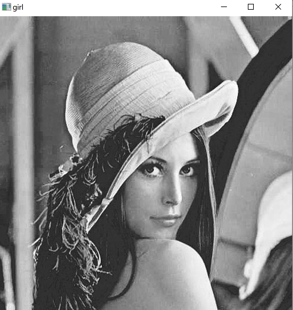
Gray conversion: convert three channels into single channel image CVT cvtColor()
g
r
a
y
=
B
×
0.114
+
G
×
0.587
+
R
∗
0.299
gray = B×0.114+G×0.587+R*0.299
gray=B×0.114+G×0.587+R∗0.299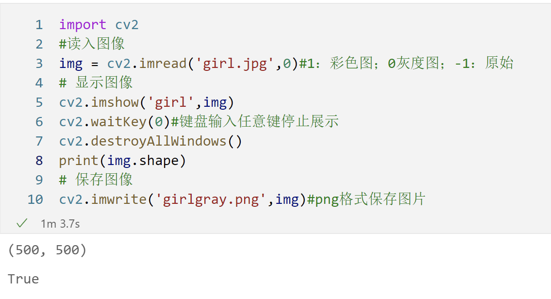
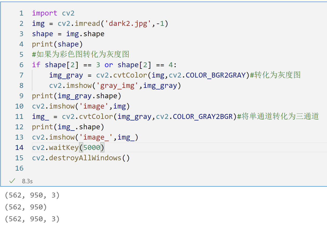
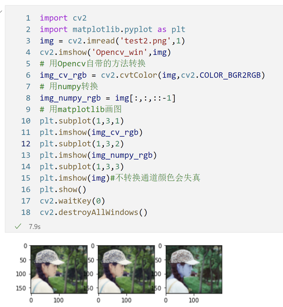
Convert BGR to RGB: when reading images with cv, they are stored in BGR order. If drawing with plot, it is necessary to convert BGR to RGB.
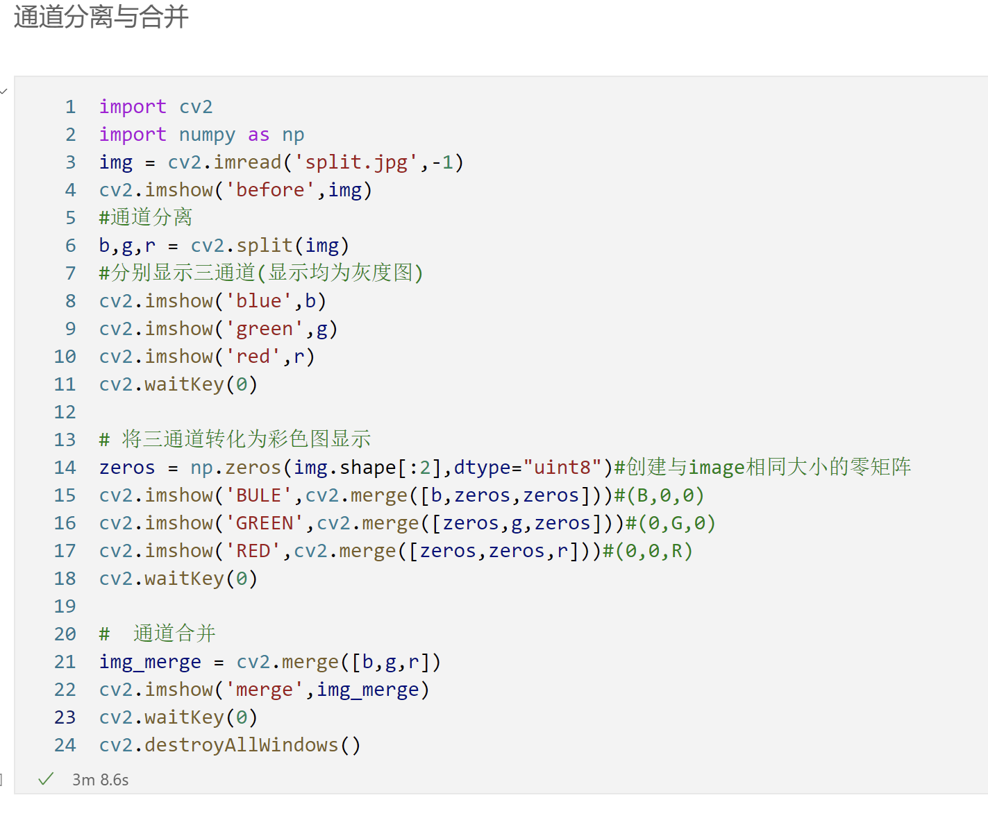
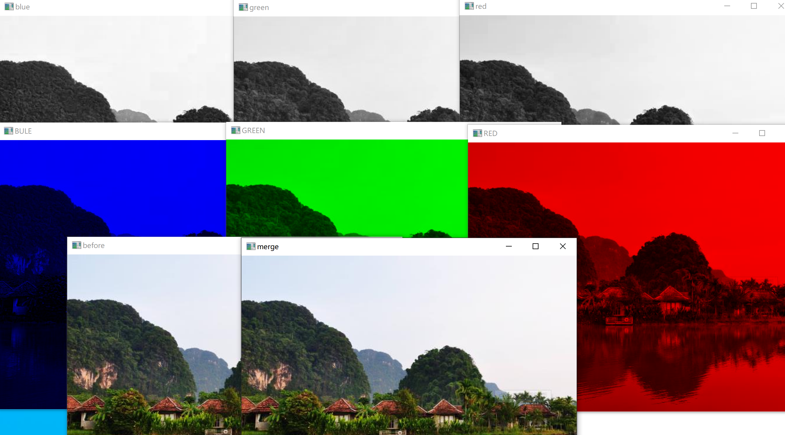
Channel separation: separate the color image into three single channel images CV2 split()
Channel merging: modify the three single channels B, G and R, and finally merge the modified single channel into a color image CV2 merge()
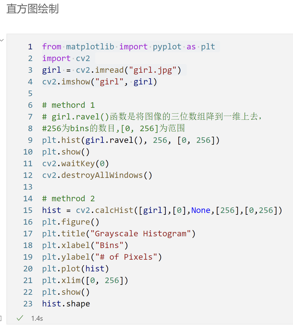
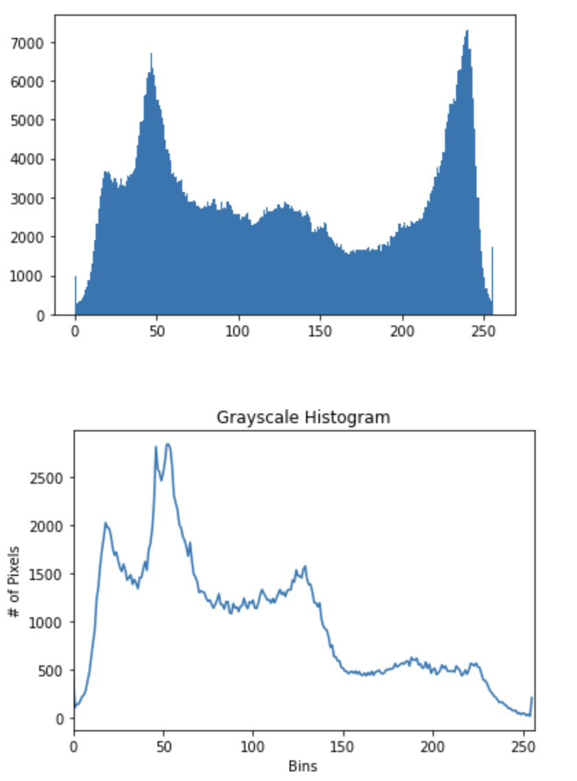
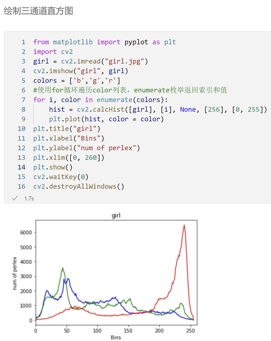
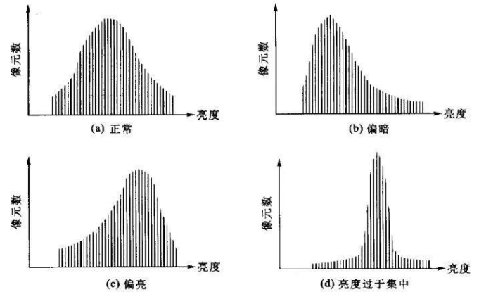
Histogram: the histogram describes the number of pixels of each brightness value in the image, and the left side is pure black and dark; The right side is bright and pure white. cv2.calcHist()
2 basic image operation
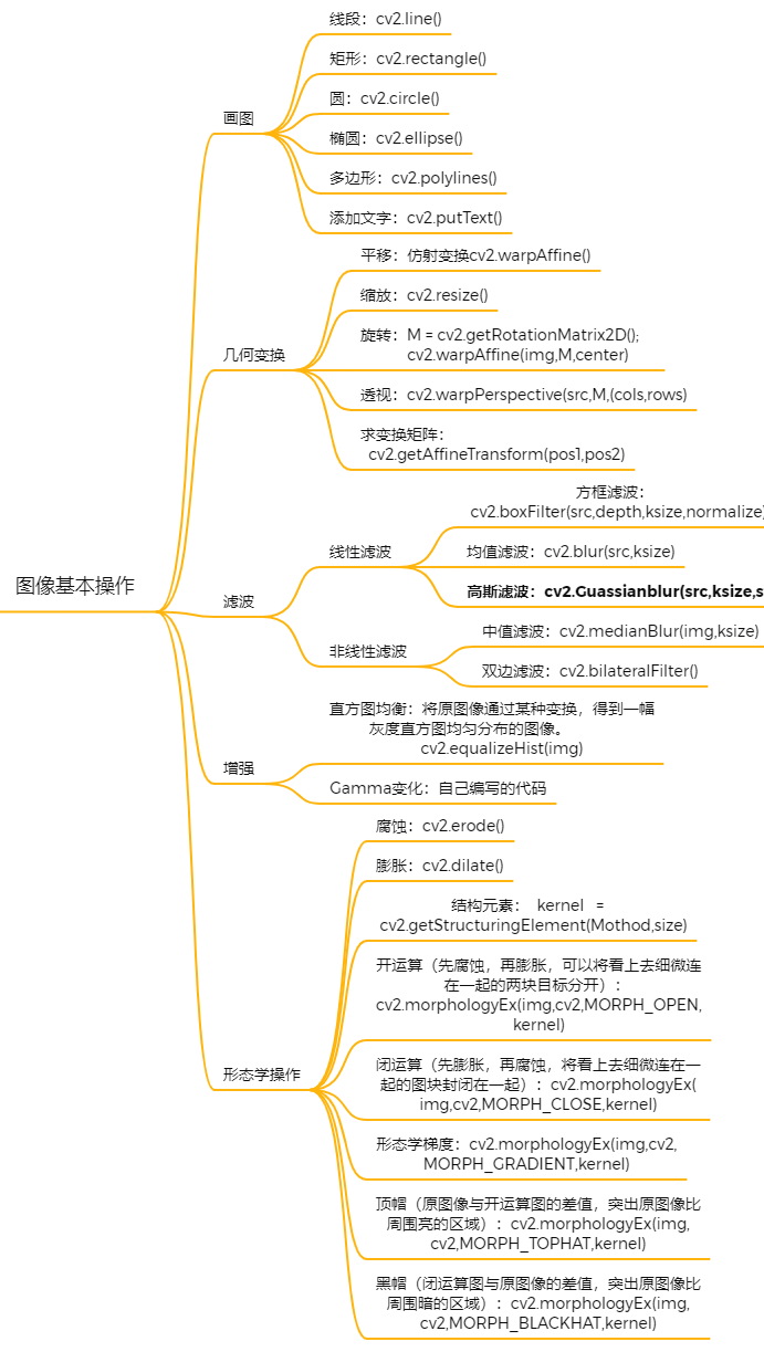
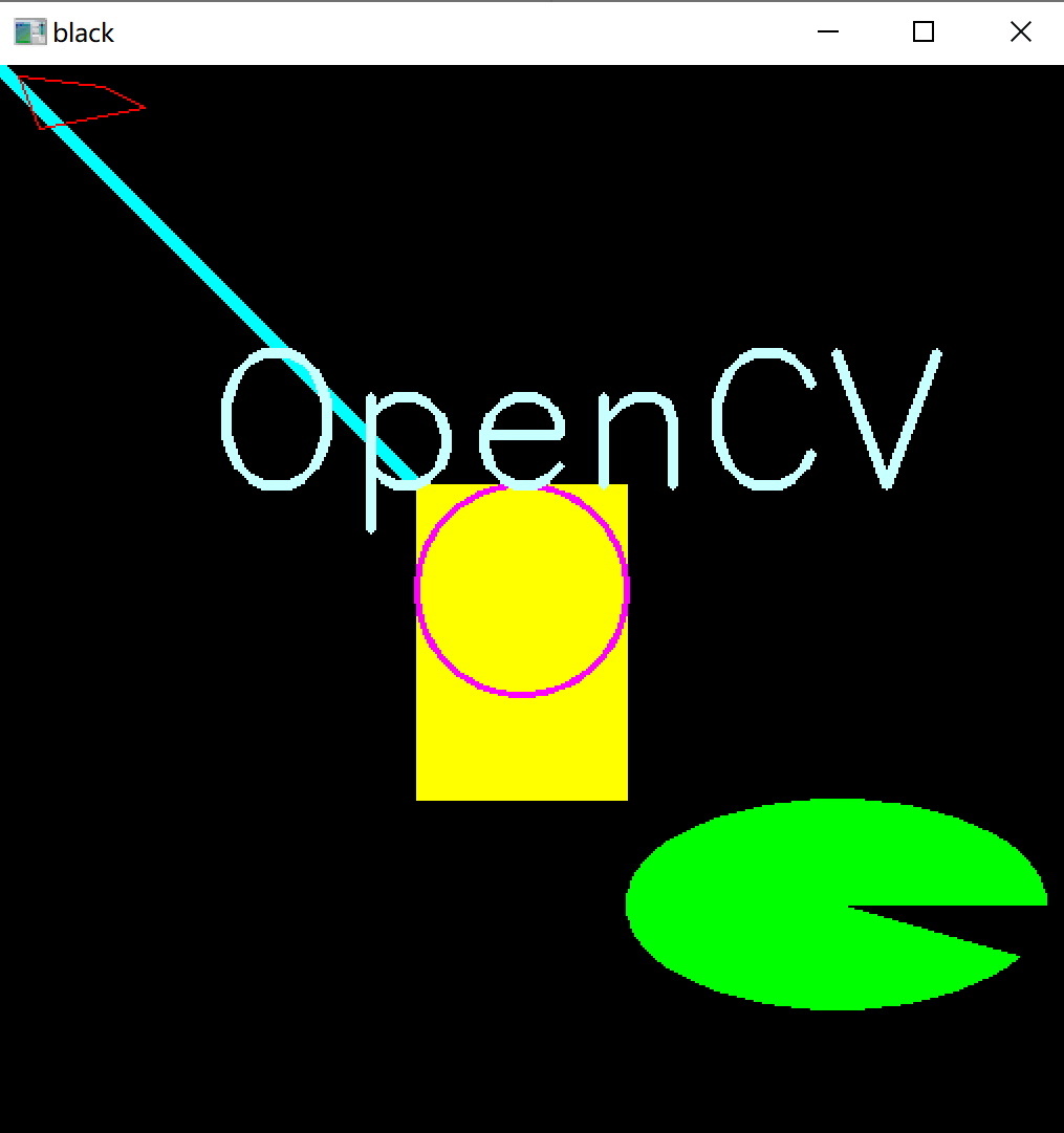
2.1 drawing
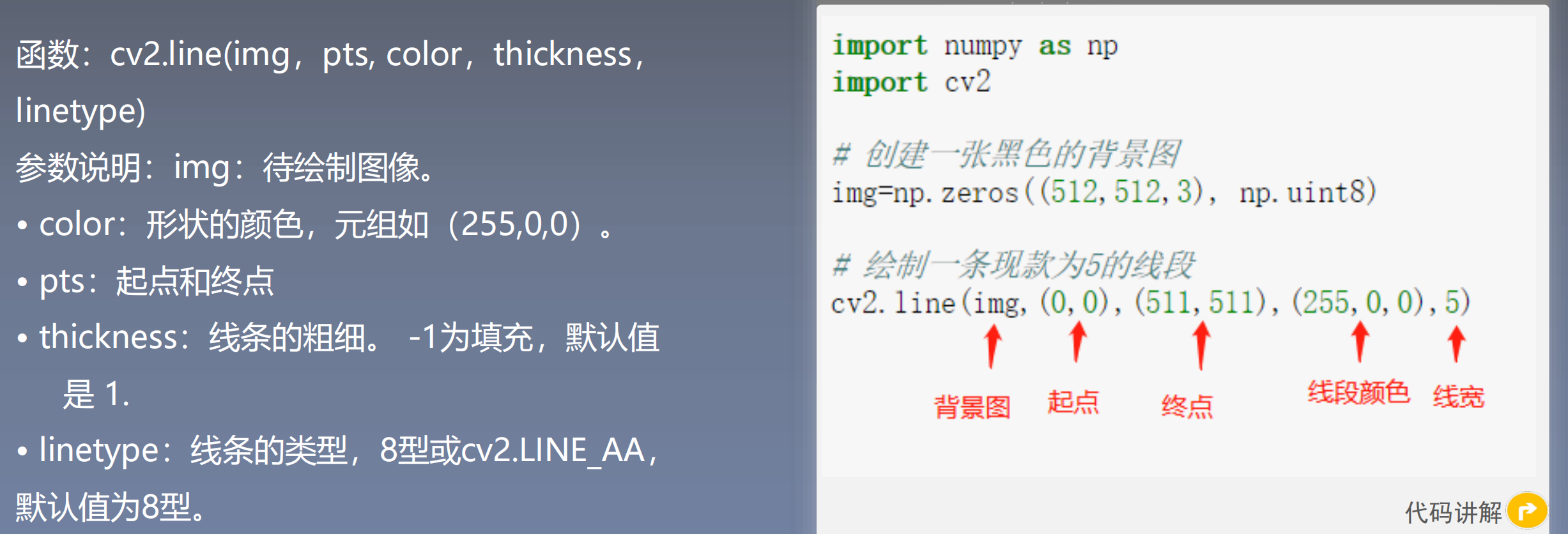
Draw line segments:
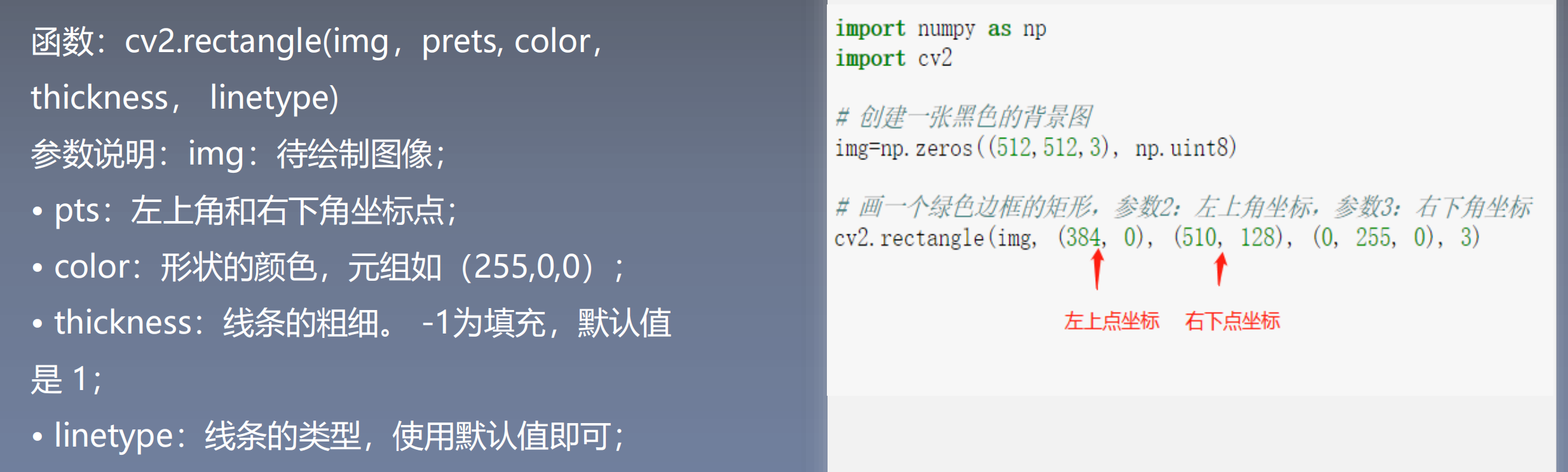
Draw rectangle:
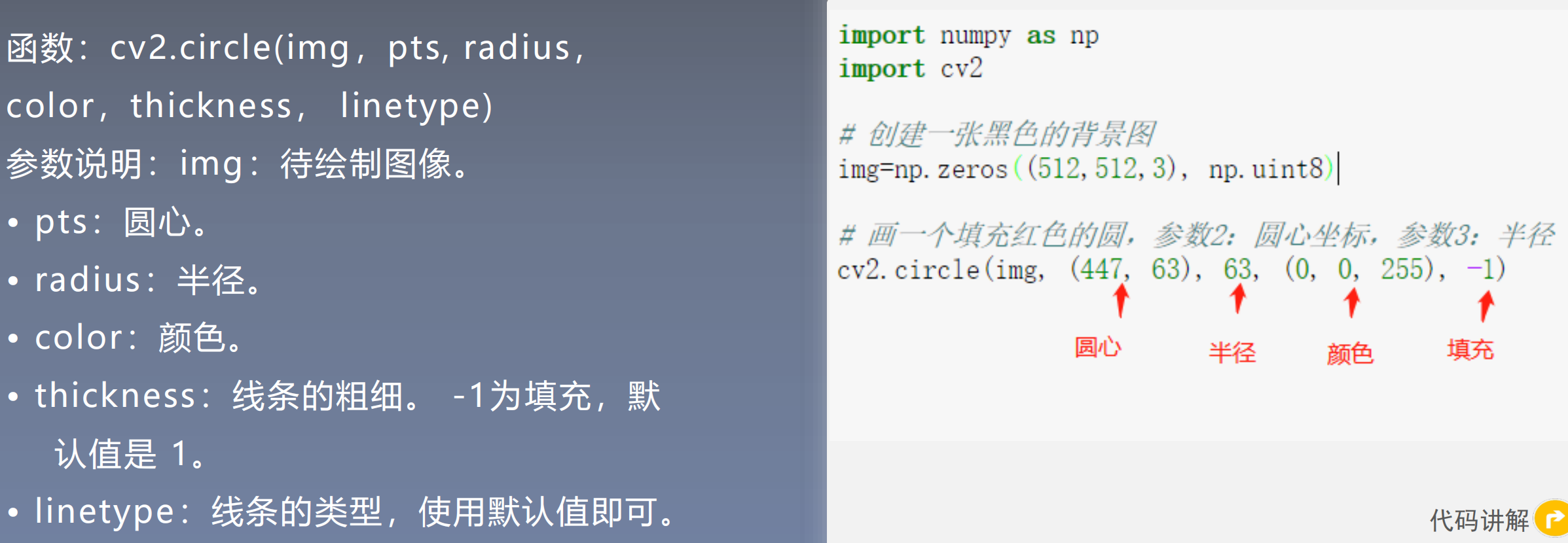
Draw circle:
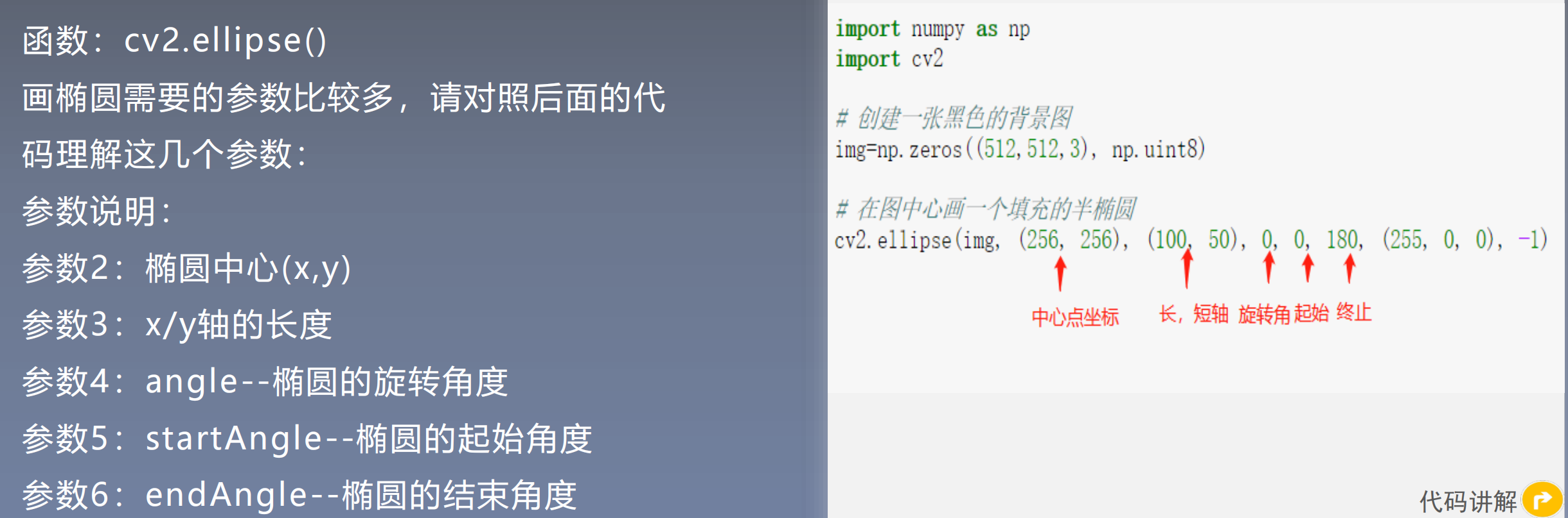
Draw ellipse:
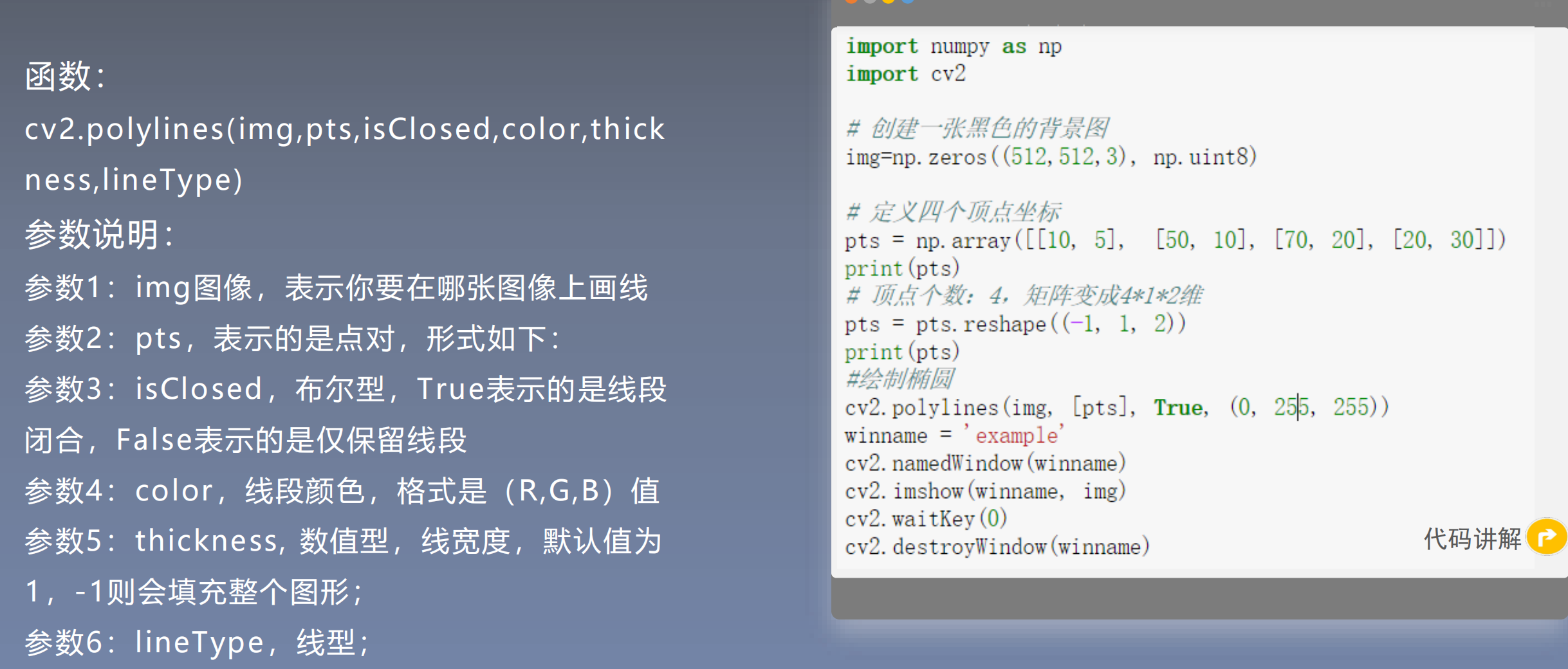
Draw polygons:
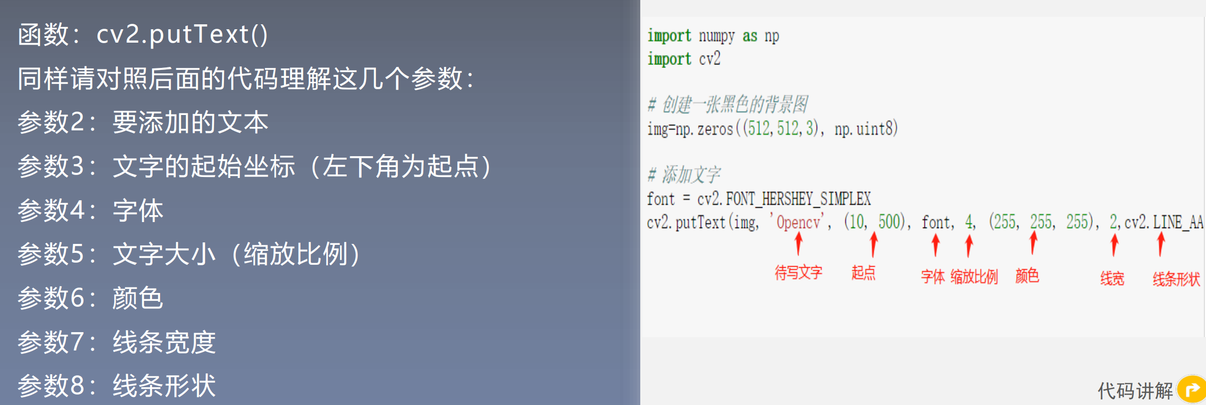
Add text:

2.2 image geometric transformation
Image pan:
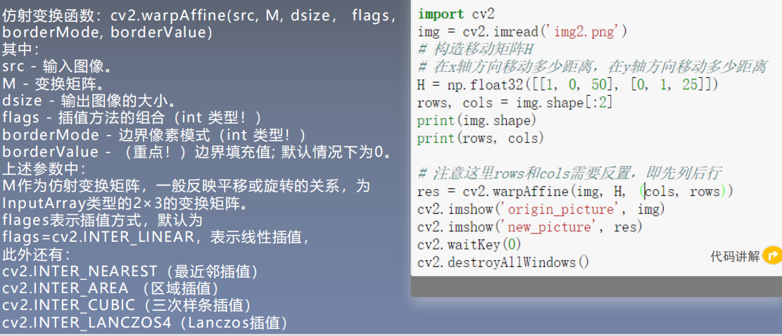
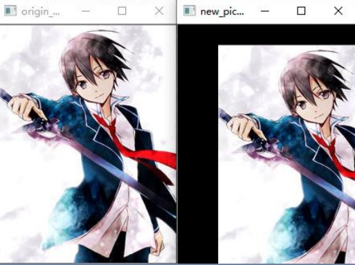
Image scaling: down sampling, up sampling.
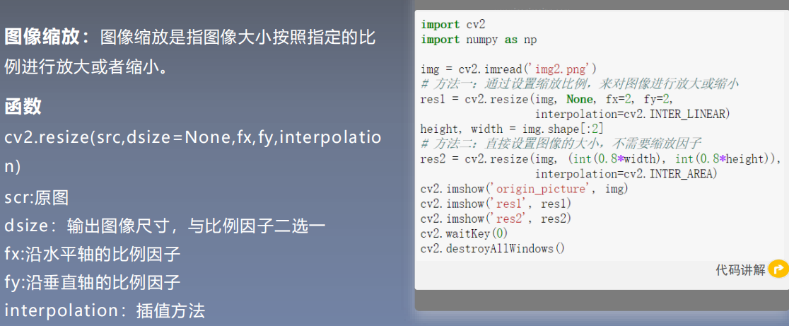
Interpolation method: nearest neighbor interpolation; Bilinear interpolation;
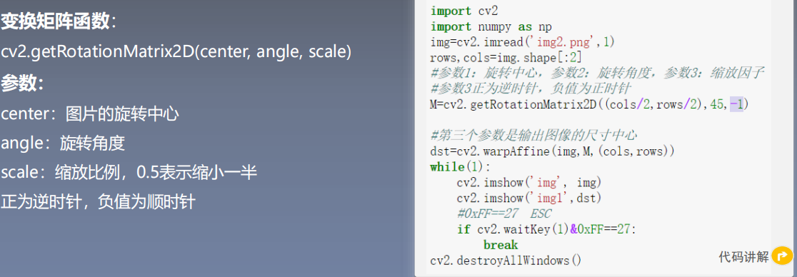
Image rotation:
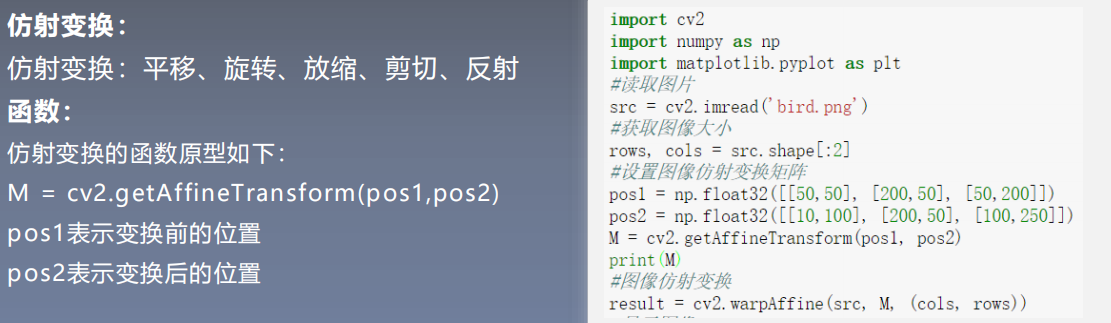
Affine transformation:
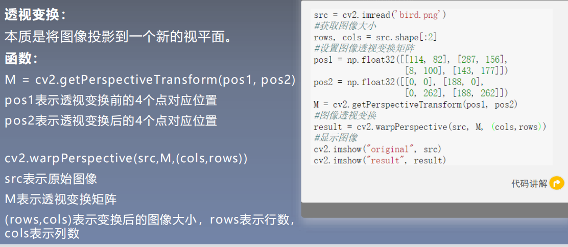
Perspective transformation:
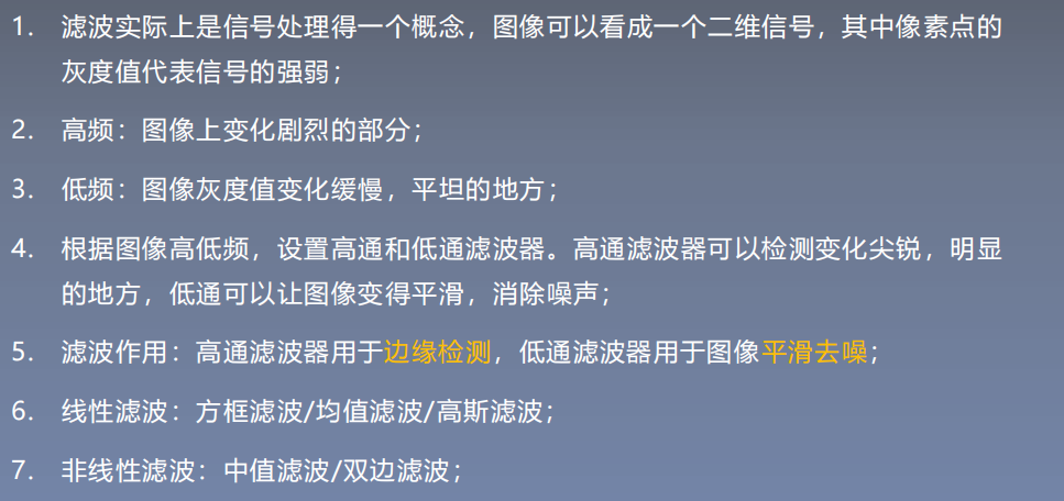
2.3 image filtering and enhancement
High pass filter is used for edge detection and low-pass filter is used for image smoothing and denoising.
Neighborhood operator: an operator whose value of pixels around a given pixel determines the final input of a given pixel. Linear filtering is a common neighborhood operator, and its pixel output value depends on the weighted sum of input pixels.
g
(
i
,
j
)
=
∑
k
,
l
f
(
i
+
k
,
j
+
l
)
h
(
k
,
l
)
g(i,j)=\sum_{k,l}f(i+k,j+l)h(k,l)
g(i,j)=k,l∑f(i+k,j+l)h(k,l) 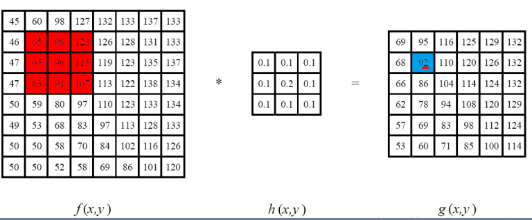
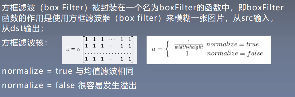
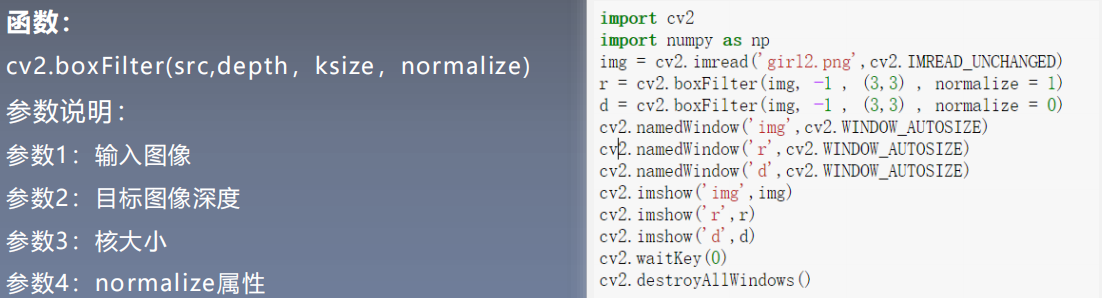
Linear filtering - block filtering:
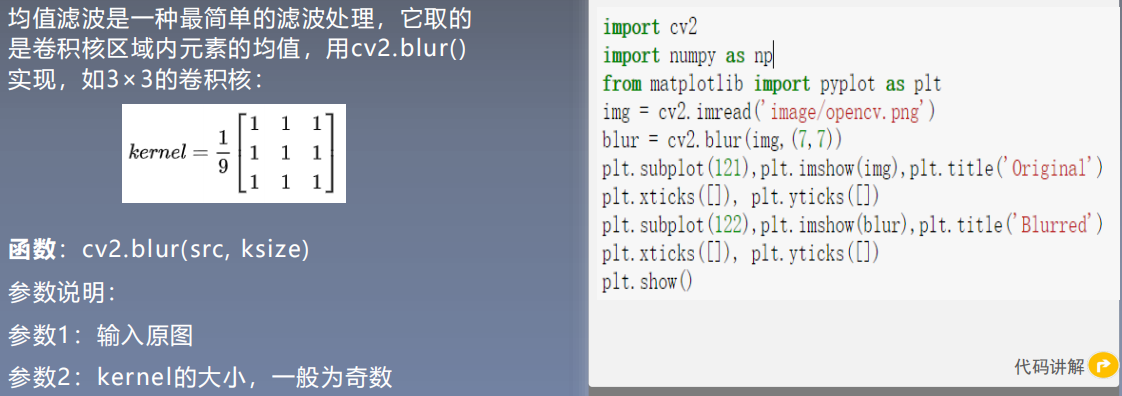
Linear filtering - mean filtering:
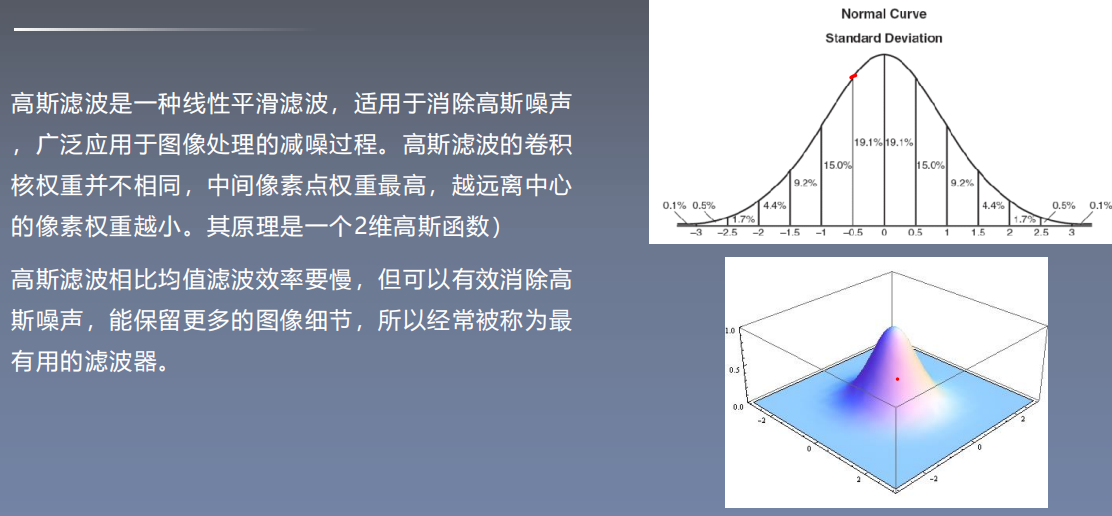
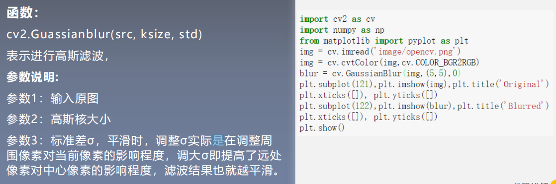
Linear filtering - Gaussian filtering:
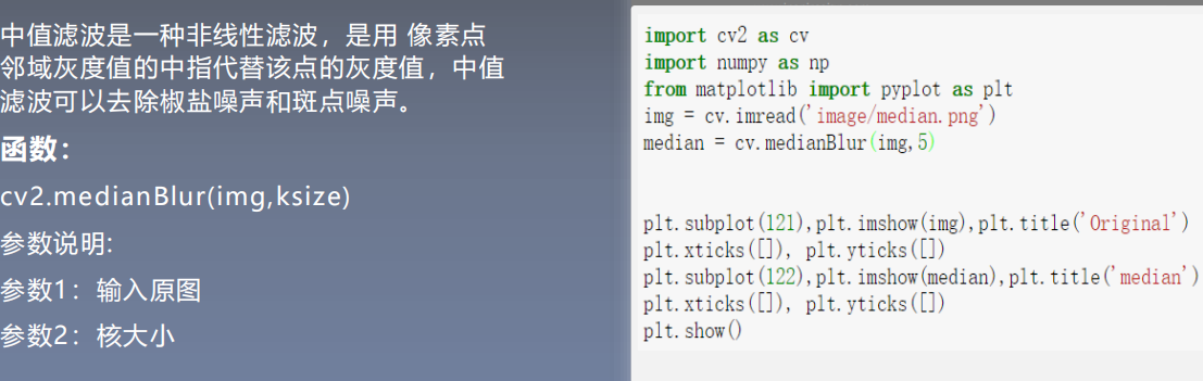
Nonlinear filtering - median filtering:
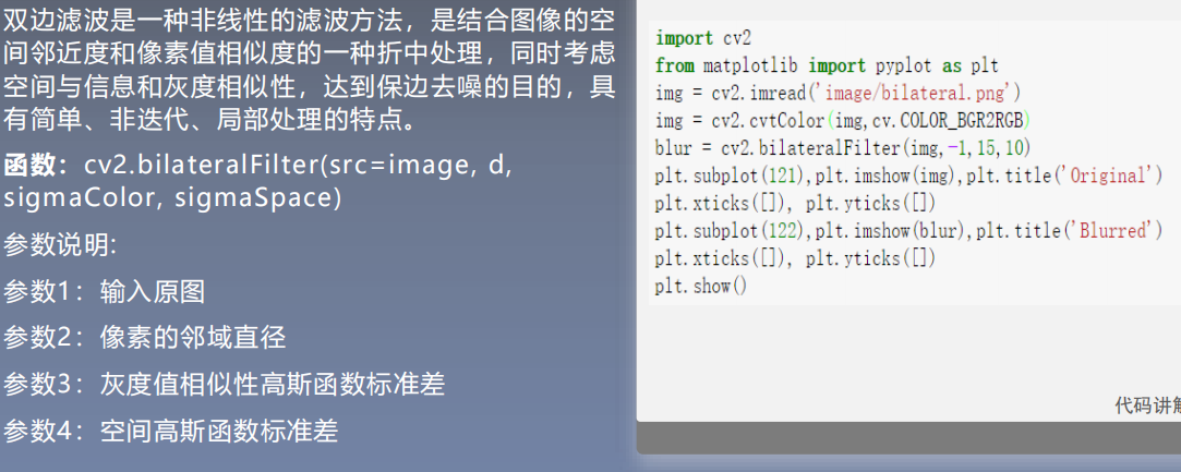
Nonlinear filtering - bilateral filtering:
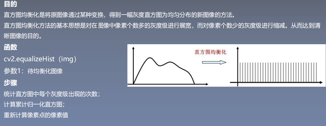
Histogram equalization
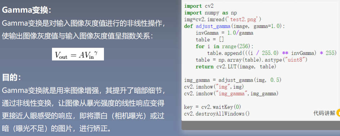
Gamma variation:
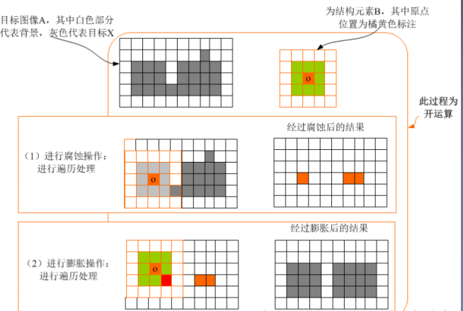
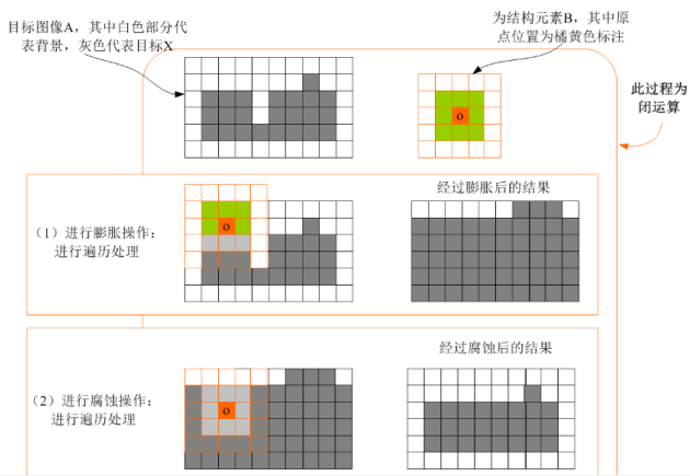
2.4 image morphological operation
Image corrosion:
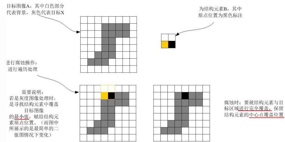
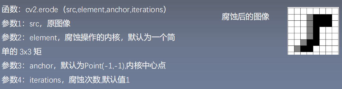
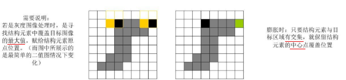
Image expansion:
Open operation: first corrosion and then expansion to separate the two finely connected targets.
Closed operation: expand first and then corrode, and close the fine connected drawings together.
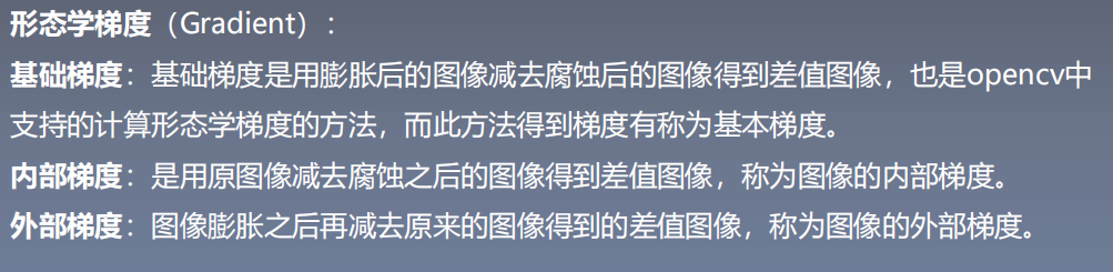
Morphological gradient:
Top hat and black hat:

3 image segmentation
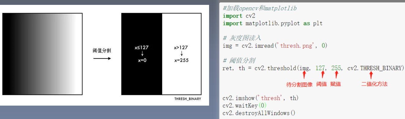
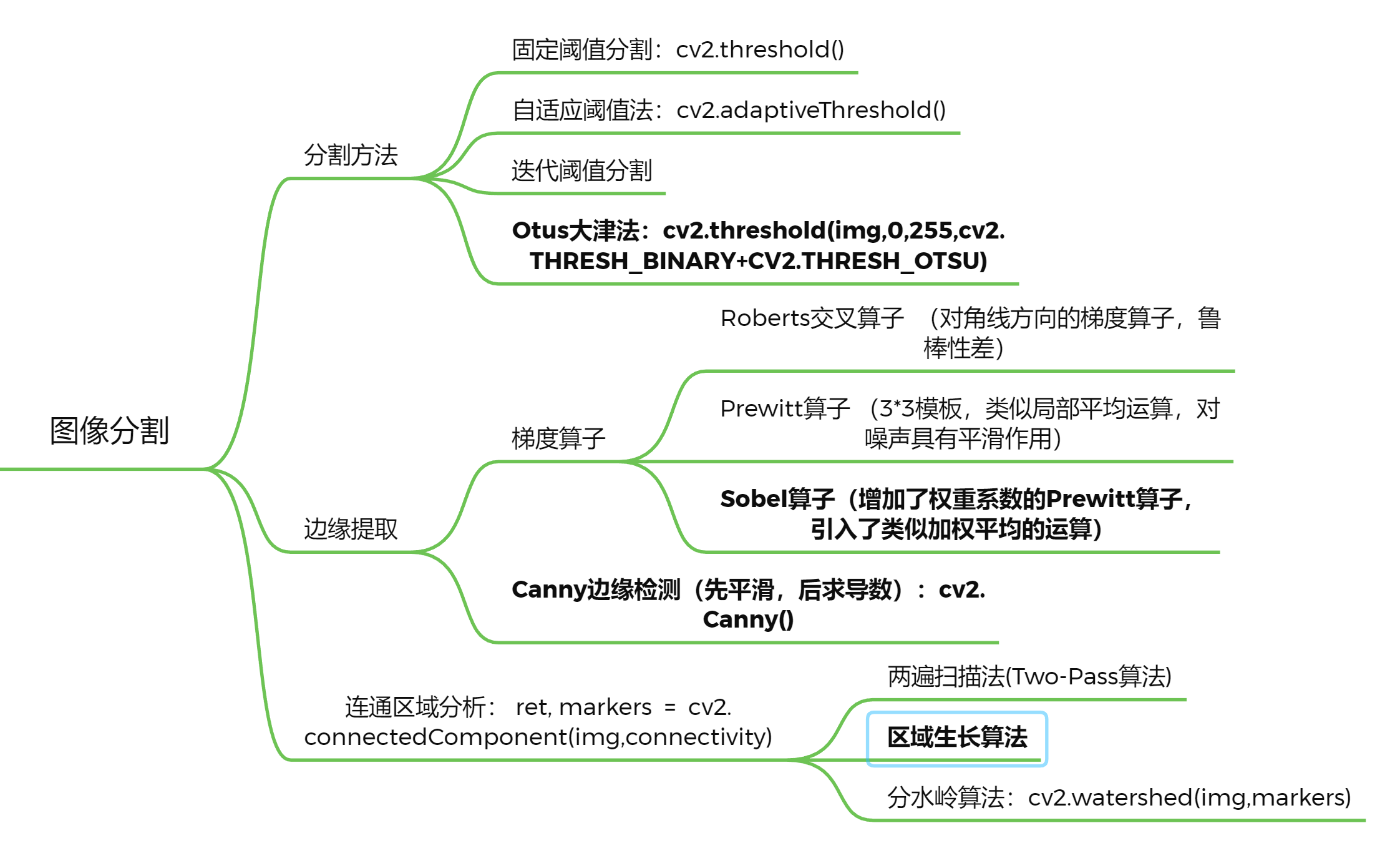 Image segmentation refers to the process of dividing several images into regions with similar properties. There are mainly image segmentation methods based on threshold, region, edge, clustering, graph theory and depth learning. Image segmentation is divided into semantic segmentation and instance segmentation. Principle of segmentation: make the divided subgraphs keep the maximum similarity internally and the minimum similarity between subgraphs## 3.1 segmentation method * * fixed threshold image segmentation * *:
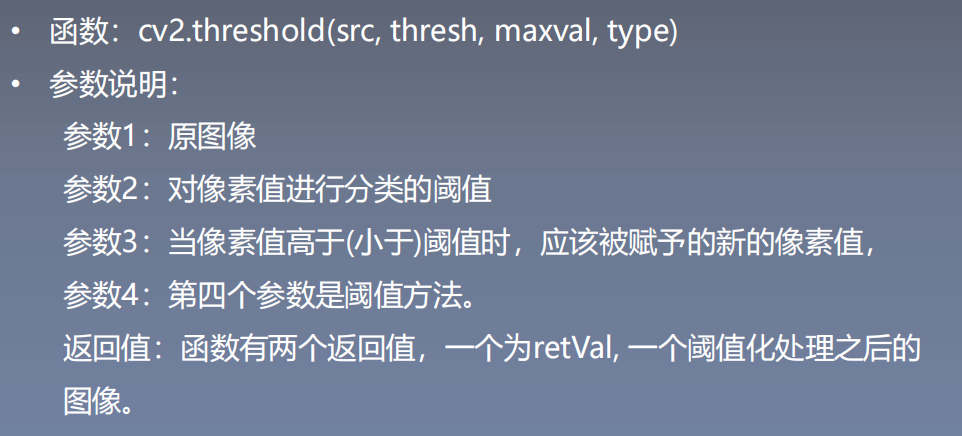
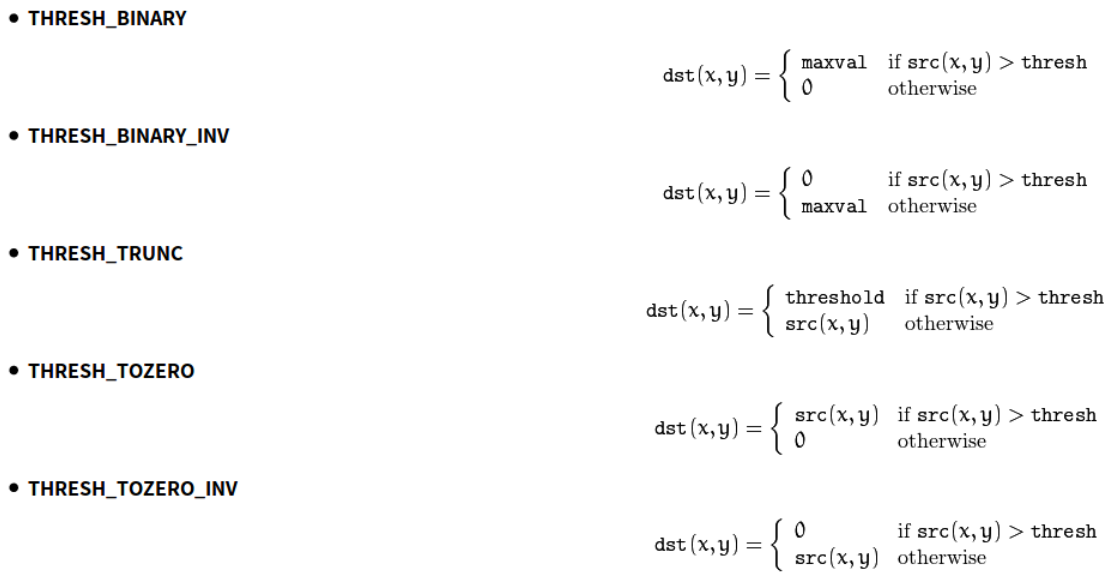
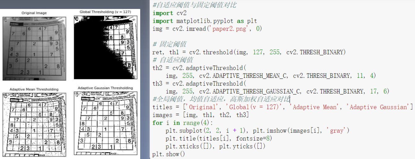
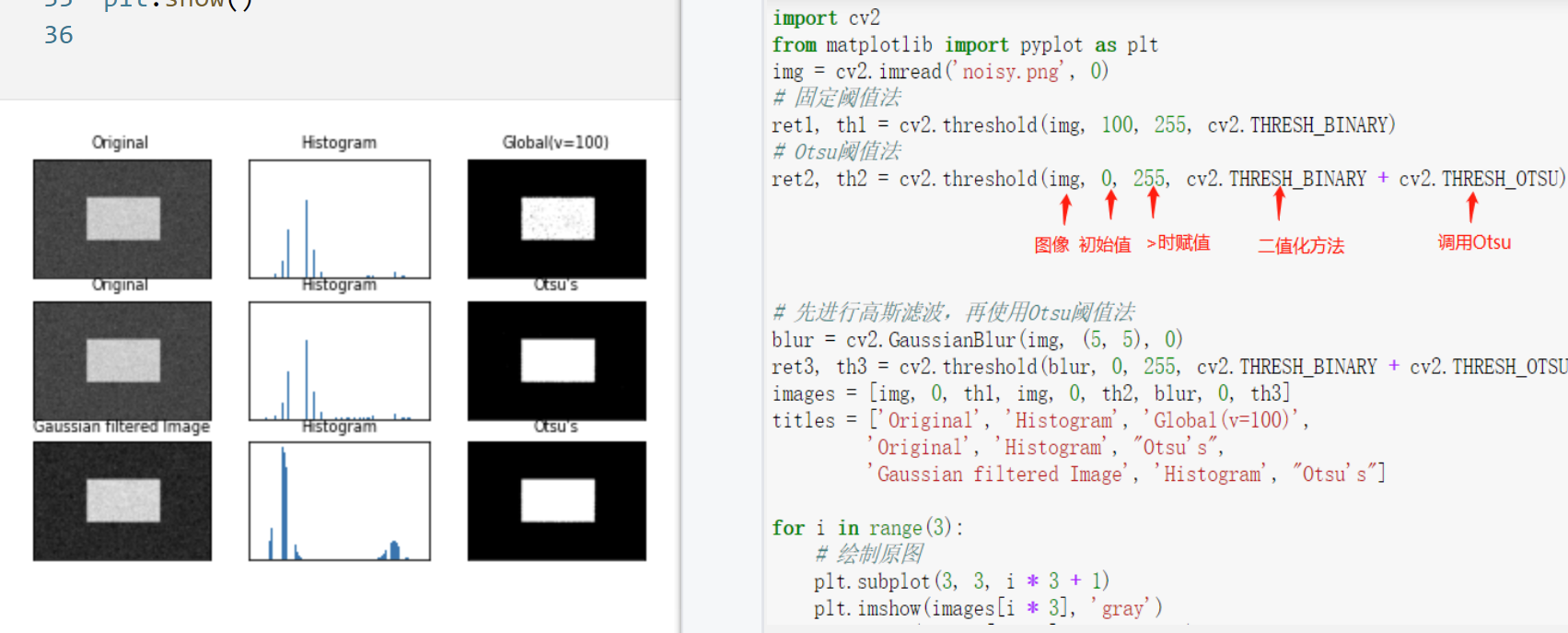
 Five threshold methods:
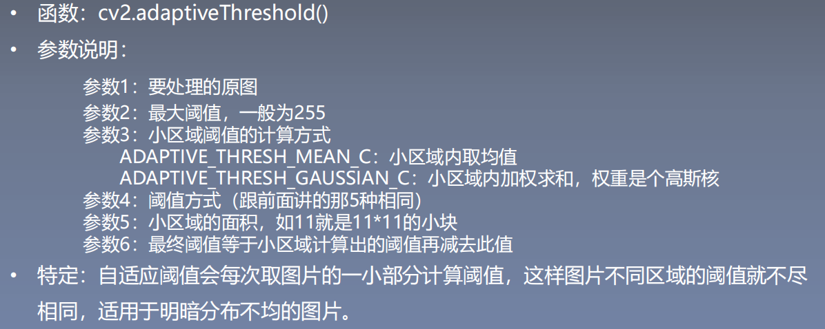
 **Automatic threshold segmentation * *:
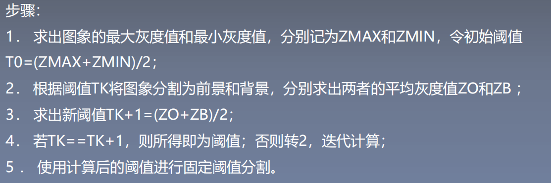
 **Iterative threshold segmentation * *:
import cv2
import numpy as np
import matplotlib.pyplot as plt
import matplotlib.cm as cm
def best_thresh(img):
img_array = np.array(img).astype(np.float32)#Convert to array
I=img_array
zmax=np.max(I)
zmin=np.min(I)
tk=(zmax+zmin)/2#Set initial threshold
print(tk)
#The image is segmented into foreground and background according to the threshold, and the average gray zo and zb are obtained respectively
b=1
m,n=I.shape
while b==1:
ifg=0
ibg=0
fnum=0
bnum=0
# Traverse every point on the image
for i in range(1,m):
for j in range(1,n):
tmp=I[i,j]
if tmp>=tk:
ifg=ifg+1
fnum=fnum+int(tmp)#The number of foreground pixels and the sum of pixel values
else:
ibg=ibg+1
bnum=bnum+int(tmp)#The number of background pixels and the sum of pixel values
#Calculate the average of foreground and background
zo=int(fnum/ifg)
zb=int(bnum/ibg)
if tk==int((zo+zb)/2):#If the average value of foreground and background is equal to the current threshold, exit the cycle
b=0
else:
tk=int((zo+zb)/2)#If not, update the threshold
return tk
img = cv2.imread("./image/bird.png")
img = cv2.cvtColor(img,cv2.COLOR_BGR2RGB)
gray = cv2.cvtColor(img,cv2.COLOR_RGB2GRAY)
img = cv2.resize(gray,(200,200))#size
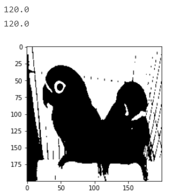
yvzhi=best_thresh(img)
ret1, th1 = cv2.threshold(img, yvzhi, 255, cv2.THRESH_BINARY)
print(ret1)
plt.imshow(th1,cmap=cm.gray)
plt.show()
result:
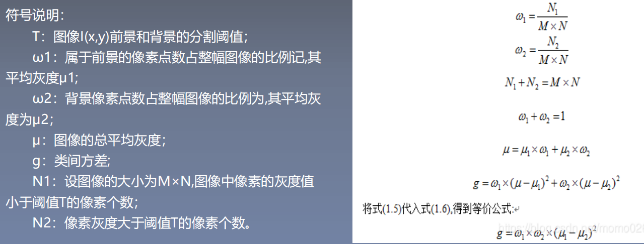
otsu Otsu otsu method: it is an adaptive method based on global threshold to maximize the inter class variance of the segmentation results.
3.2 edge extraction
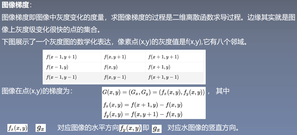
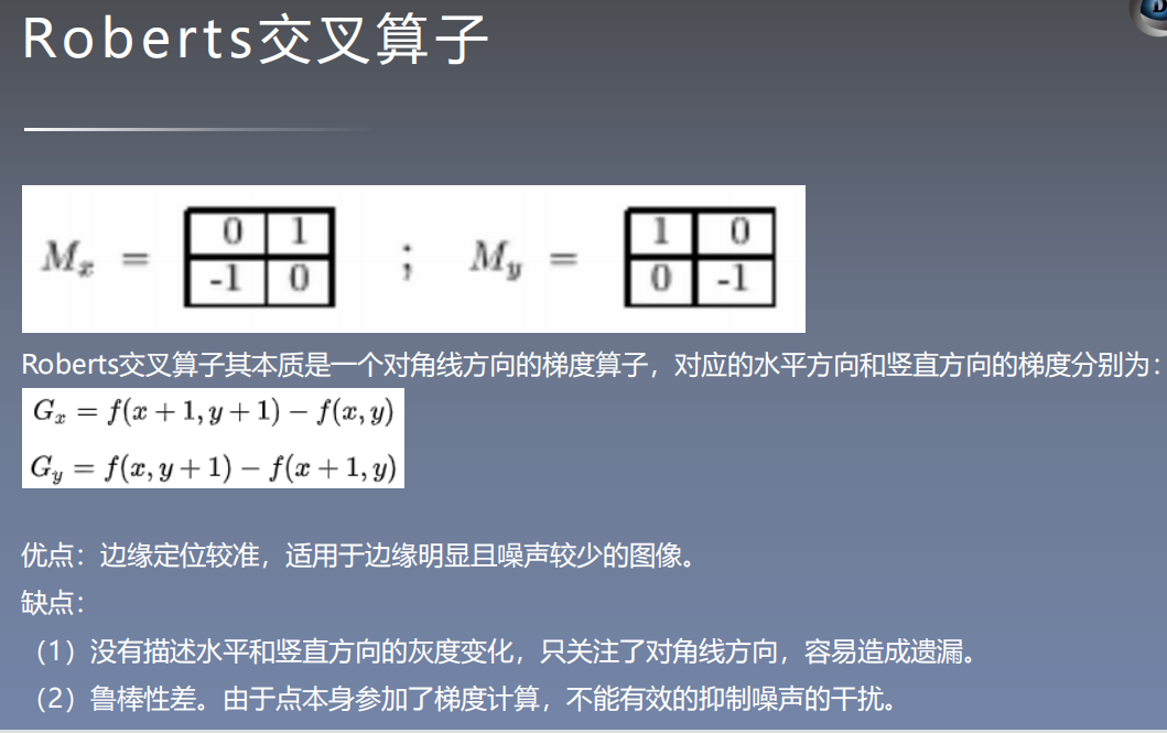
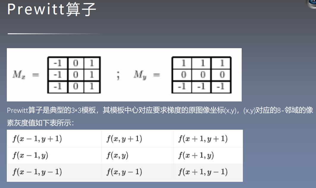
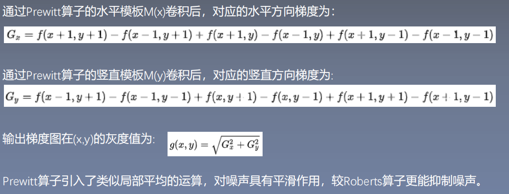
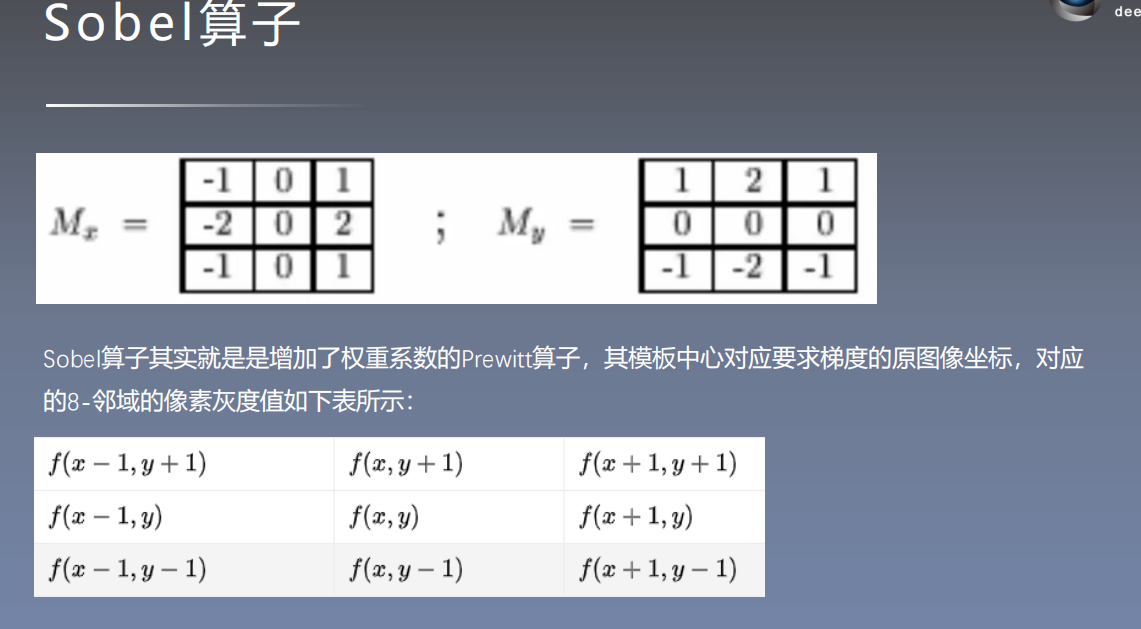
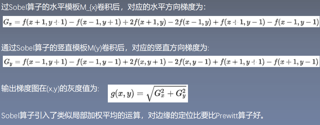
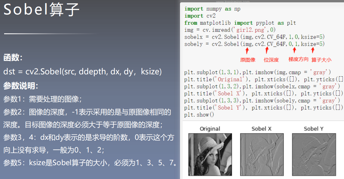
Image gradient:
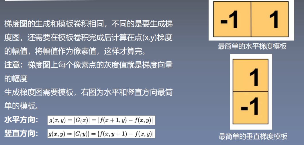
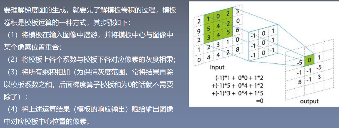
Template convolution:
Gradient operator: it is a first derivative operator
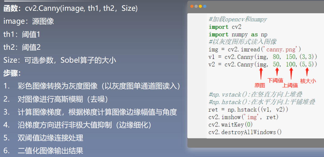
Canny edge detection algorithm: smoothing before derivation
Performance evaluation index of edge detection:
- Good signal-to-noise ratio, that is, the probability of judging non edge points as edge points is low, and the probability of judging edge points as non edge points is low;
- High positioning performance, that is, the detected edge points should be in the center of the actual edge as far as possible;
- There is only one response to a single edge, that is, the probability of multiple responses from a single edge is low, and the false response edge should be suppressed to the greatest extent.
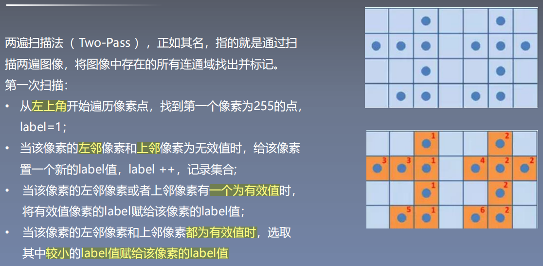
3.3 connected area analysis
Two pass algorithm:
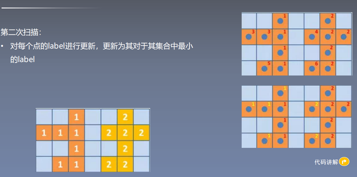
Code implementation:
Tow pass code
Region growth algorithm:
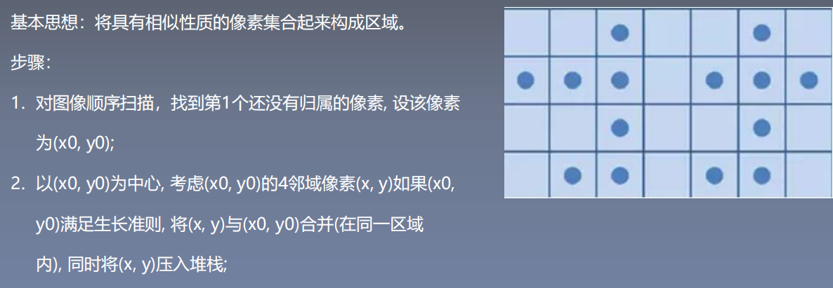
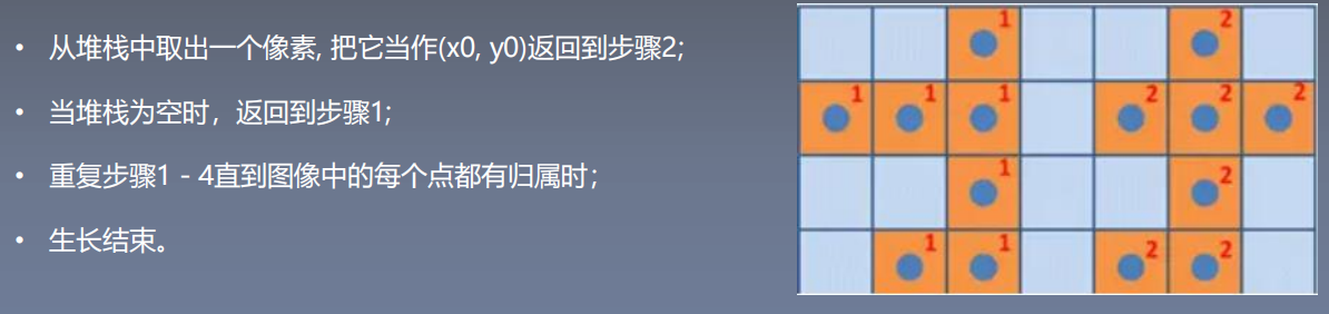
The decisive factors of regional growth are: the selection of initial point (seed point), growth criteria and termination conditions.
Code implementation:
Region growth Code
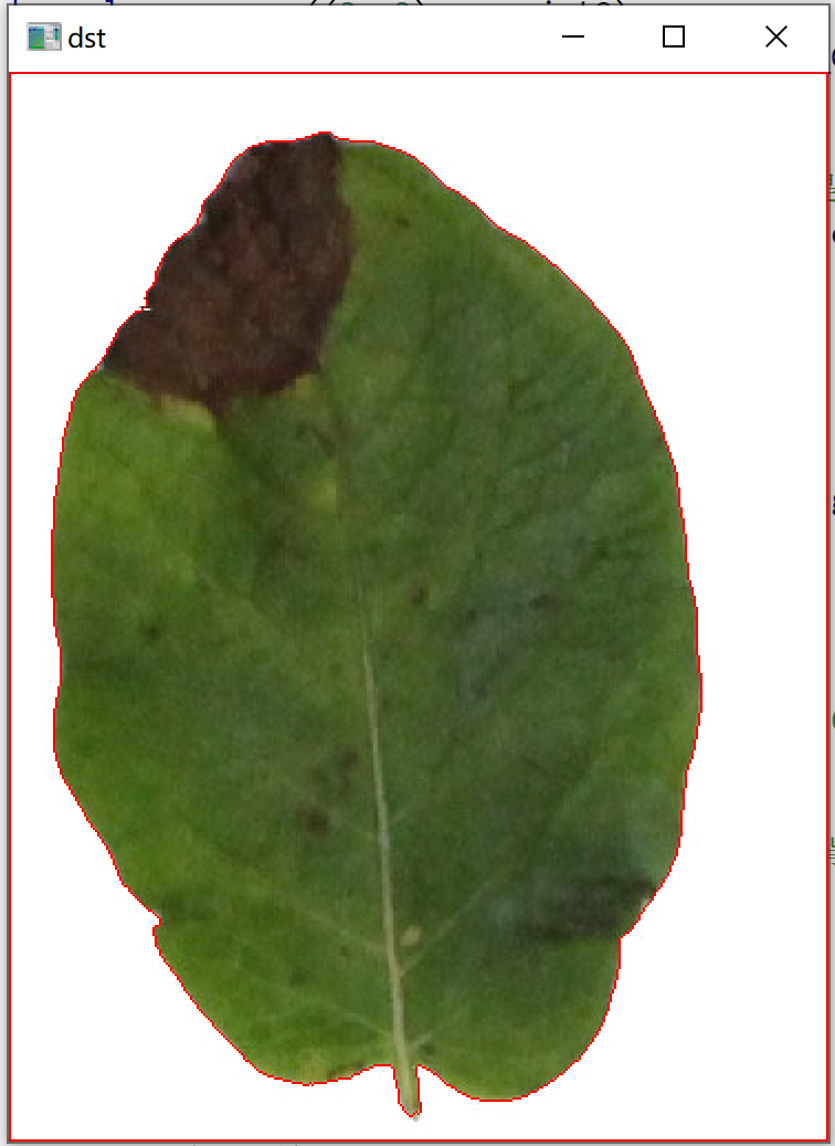
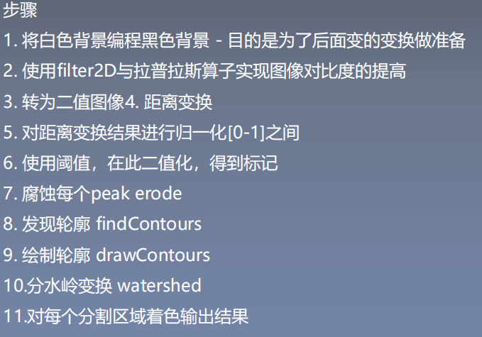
Watershed algorithm: give each isolated valley (local minimum) different colors of water (labels). When the water rises, different valleys, that is, different colors will begin to merge according to the surrounding peaks (gradients). To avoid Valley merging, a watershed needs to be established where the water needs to merge until all peaks are submerged, The created watershed is the dividing boundary line, which is the principle of watershed.
# import cv2
"""
Complete the steps of watershed algorithm:
1,Load original image
2,Threshold segmentation, the image is divided into black and white parts
3,Open the image, that is, first corrosion in expansion
4,The result of the split operation is expanded to obtain most of the area that is the background
5,Through distance transformation Distance Transform Get foreground area
6,Background area sure_bg And foreground area sure_fg By subtraction, the overlapping area with both foreground and background is obtained
7,Connected area processing
8,Finally, watershed algorithm is used
"""
import cv2
import numpy as np

# Step1.  Load image
img = cv2.imread('image/yezi.jpg')
cv2.imshow("img", img)
cv2.waitKey(0)
cv2.destroyAllWindows()
gray = cv2.cvtColor(img, cv2.COLOR_BGR2GRAY)
# Step2. Threshold segmentation divides the image into black and white parts
ret, thresh = cv2.threshold(gray, 0, 255, cv2.THRESH_BINARY_INV + cv2.THRESH_OTSU)
# cv2.imshow("thresh", thresh)

# Step3.  Carry out "open operation" on the image, corrode first and then expand
kernel = np.ones((3, 3), np.uint8)
opening = cv2.morphologyEx(thresh, cv2.MORPH_OPEN, kernel, iterations=2)
# cv2.imshow("opening", opening)

# Step4.  Expand the result of the "open operation" to obtain the area most of which is the background
sure_bg = cv2.dilate(opening, kernel, iterations=3)
cv2.imshow("sure_bg", sure_bg)
cv2.waitKey(0)
cv2.destroyAllWindows()

# Step5. Get foreground area through distanceTransform
dist_transform = cv2.distanceTransform(opening, cv2.DIST_L2, 5)  # DIST_L1 DIST_C can only correspond to mask 3 dist_ L2 can be 3 or 5
cv2.imshow("dist_transform", dist_transform)
cv2.waitKey(0)
cv2.destroyAllWindows()
print(dist_transform.max())
ret, sure_fg = cv2.threshold(dist_transform, 0.1 * dist_transform.max(), 255, 0)

# Step6. sure_bg And sure_fg subtract ,The overlapping region with both foreground and background is obtained   #The relationship between this area and the contour area is unknown
sure_fg = np.uint8(sure_fg)
unknow = cv2.subtract(sure_bg, sure_fg)
cv2.imshow("unknow", unknow)
cv2.waitKey(0)
cv2.destroyAllWindows()

# Step7.  Connected area processing
ret, markers = cv2.connectedComponents(sure_fg,connectivity=8) #Label the connected area, and the sequence number is 0 - N-1
#print(markers)
print(ret)
markers = markers + 1           #OpenCV watershed algorithm must label objects greater than 1, and the background label is 0. Therefore, adding 1 to all markers becomes 1 - n
#Remove the part belonging to the background area (i.e. make it 0 and become the background)
# The Python syntax of this statement is similar to if, "unknown = = 255" returns the truth table of the image matrix.
markers[unknow==255] = 0

# Step8. watershed algorithm
markers = cv2.watershed(img, markers)  #After the watershed algorithm, the pixels of all contours are marked as - 1
#print(markers)

img[markers == -1] = [0, 0, 255]   # Pixels marked with - 1 are marked in red
cv2.imshow("dst", img)
cv2.waitKey(0)
cv2.destroyAllWindows()
result: