catalogue

Competitive game problem

1.1 problem transformation

1.2 Nash equilibrium

1.3 KKT equivalence between optimization problem and equilibrium problem

2 compact model

3 GAMS source code for solving MCP model with PATH solver

3.1 source code file

3.2 calculation results

List of published articles in this series:

Lecture01: optimal modeling of market clearing problem

Lecture1b: how to get the optimal conditions and dual problems from the primitive linear programming model

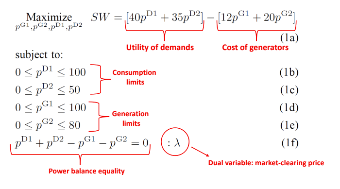
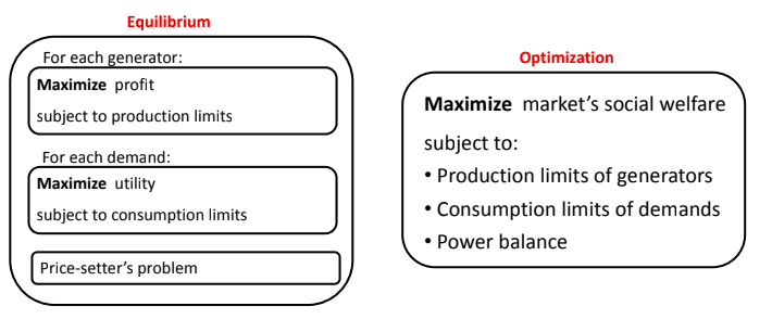
Review the previous problem model of electricity market:

Competitive game problem

1.1 problem transformation

For power plants, the goal is to maximize revenue; For power enterprises, it is to maximize utility. So, how to calculate the benefits and utility?

• Power plant Revenue: power generation * (market price - power generation cost price)
• Utility of power users: electricity consumption * (bidding price - market price)

Therefore, for each market participant, we have the following optimization problems:

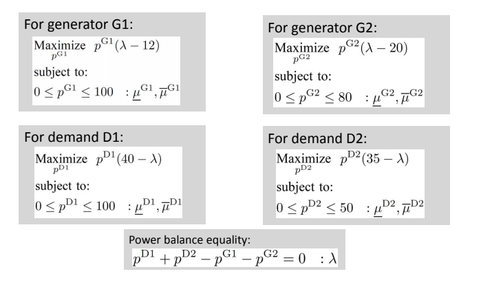
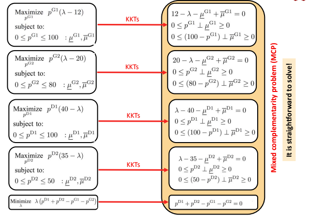
According to the KKT condition, we can equivalent the power balance constraint to an optimization problem:

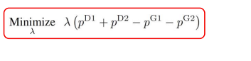
In this optimization problem, we try to punish any mismatch between supply and demand. In other words, if the production price is not equal to the demand price, there will be λ Punishment.

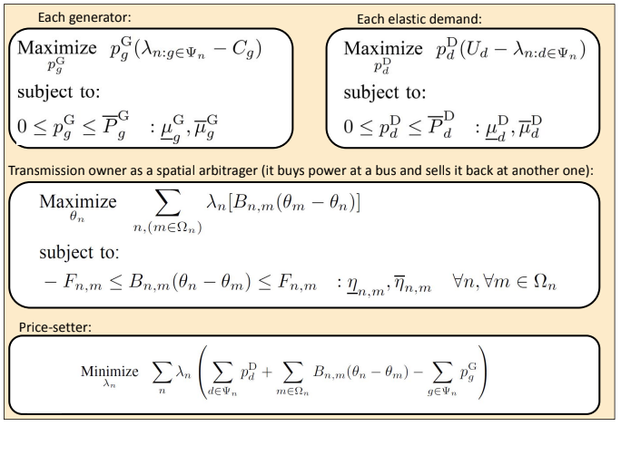
Thus, we get five optimization problems:

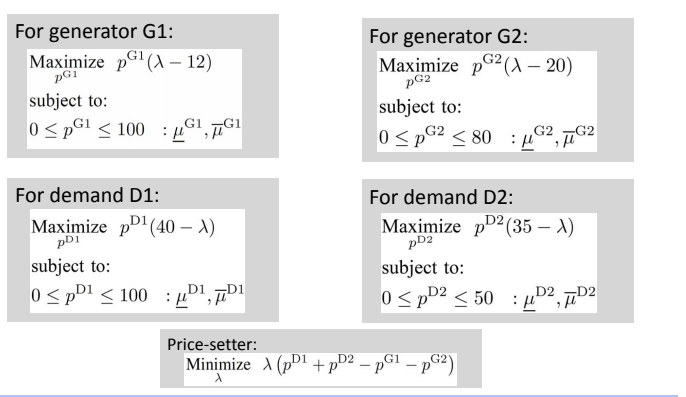
So can we solve these five problems separately? Obviously not. as a result of:

• Market clearing price λ In the price setter problem, it is a variable, while in G1, G2, D1 and D2, it is a parameter
• Power generation and consumption are variables in G1, G2, D1 and D2, and parameters in price setter problem
• Therefore, the above five issues are interrelated, and we cannot disassemble them and deal with them separately. This is a game theory problem.

This problem is also called "competitive equilibrium", which is a non cooperative game. All players are pursuing their own maximum interests. Only when they maximize the interests of the alliance as an alliance can they build a cooperative game.

Three classic literatures on competitive game:

1. Kantorovich, L. V. (1960). Mathematical methods of organizing and planning production. Management science, 6(4), 366-422.
2. Samuelson, P. A. (1952). Spatial price equilibrium and linear programming. The American economic review, 42(3), 283-303.
3. Arrow, K. J., & Debreu, G. (1954). Existence of an equilibrium for a competitive economy. Econometrica: Journal of the Econometric Society, 265-290.

1.2 Nash equilibrium

Nash equilibrium: no market participant can deviate from the equilibrium point and increase his own interests

Constraints depend only on themselves, while goals are associated with other participants. Such a problem can be called a Nash equilibrium problem. In the generalized Nash equilibrium problem, the objectives and constraints of each participant are associated with other parameters. Obviously, our problem is a Nash equilibrium, but not a generalized Nash equilibrium.

We discuss Nash equilibrium and generalized Nash equilibrium, so why distinguish them? Because Nash equilibrium has many good properties, such as the existence and uniqueness of solutions; The generalized Nash equilibrium does not have the same excellent properties.

So, how can all participants be satisfied with the market clearing price and unwilling to violate it? We have at hand to calculate the Nash equilibrium and get the solution of the problem through optimization. In practice, which method should we adopt?

Firstly, we discuss the equilibrium method. Firstly, we use KKT condition to transform the optimization problem to obtain an MCP; Then use solvers such as PATH to calculate, or define auxiliary goals to solve.

1.3 KKT equivalence between optimization problem and equilibrium problem

Then comes the question, is the KKT obtained by the equilibrium model equivalent to the KKT obtained by the optimization model? If equivalent, then the equilibrium model and the optimization model are equivalent. Obviously, it is equivalent here.

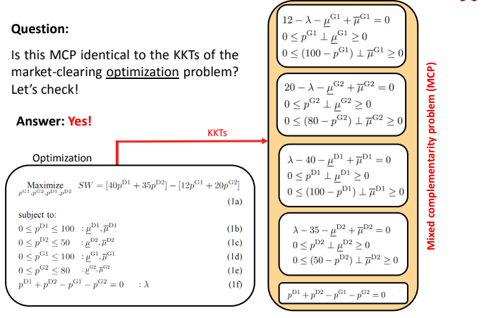
So, when we solve an optimization problem, we are actually solving an equivalent equilibrium problem. Therefore, we can draw the following two conclusions:

• Optimization problem and equilibrium problem are equivalent because they can deduce the same KKT conditions
• Both the optimization problem and the equilibrium problem can obtain the Nash equilibrium solution, that is, no market participant is willing to deviate from the market clearing price.

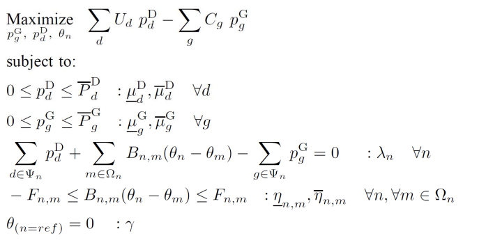
2 compact model

Optimized model version:

Equilibrium model version:

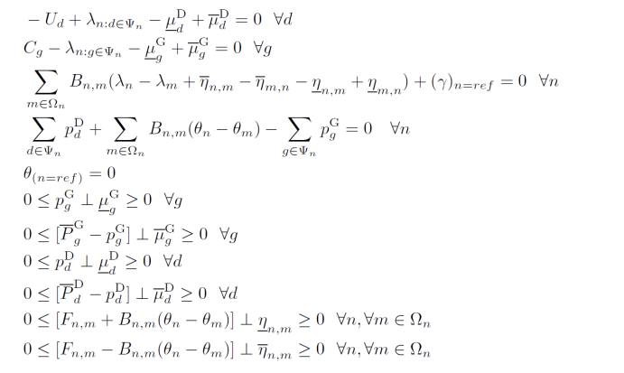
MCP model version:

3 GAMS source code for solving MCP model with PATH solver

3.1 source code file

sets
g   generators /G1*G2/
n   buses  /N1*N3/
d   demands   /D1*D2/
alias(n,m)

Sets
MapN(n,n) Network topology /
N1.N2
N1.N3
N2.N3
N2.N1
N3.N1
N3.N2/
MapG(g,n) Location of generators /
G1.N1
G2.N2/
MapD (d,n) Location of demands /
D1.N2
D2.N3/;

Parameter PGmax(g) Capacity of generators [MW]/
G1 100
G2 80/ ;
Parameter C(g) offer price of generators [$ per MWh]/
G1  12
G2  20/;
Parameter L(d) Maximum load of demands [Mw]/
D1  100
D2  50/;
Parameter U(d) utility of demands [$ per MWh]/
D1  40
D2  35/;

Table Fmax (n,n) capacity of transmission lines [MW]
    N1  N2  N3
N1  0   100 100
N2  100 0   100
N3  100 100 0;

Table B(n,n) susceptance of transmission lines [Ohm^{-1}]
    N1  N2  N3
N1  0   500 500
N2  500 0   500
N3  500 500 0;

free variable
p_D(d) consumption level of demand d [MW]
p_G(g) Production level of generator g[Mw]
theta(n) voltage angle of bus n [rad]
lambda(n) Dual var.: locational marginal price [$ per MWh]
gamma Dual var. associated with equality constraint introducing ref. bus
;

Positive variable
mu_D_min(d) Dual var. associated with lower bound of consumption level
mu_D_max(d) Dual var. associated with upper bound of consumption level
mu_G_min(g) Dual var. associated with lower bound of production level
mu_G_max(g) Dual var. associated with upper bound of production level
eta_min(n,m) Dual var. associated with transmission capacity constraints
eta_max(n, m) Dual var. associated with transmission capacity constraints;

Equations
cons1,cons2,cons3,cons4,cons5,cons6,cons7, cons8,cons9,cons10,cons11,cons12;
* Primer constraints
cons1(g).. p_G(g)=g= 0;
cons2(g).. - p_G(g) =g=-PGmax(g);
cons3(d).. p_D(d) =g= 0;
cons4(d).. - p_D(d) =g= -L(d);
cons5(n,m).. [B(n,m)*(theta(n)-theta(m))] =g= -Fmax(n,m);
cons6(n,m).. -[B(n,m)*(theta(n)-theta(m))] =g= -Fmax(n,m);
cons7.. theta('N1') =e= 0 ;
cons8(n).. - sum(g$MapG(g,n),p_G(g)) + sum(d$MapD(d,n),p_D(d))
           + sum(m$MapN(n,m),B(n,m)*(theta(n)-theta(m))) =e= 0;
* KKT conditions
cons9(d).. -U(d)+sum(n$MapD(d,n),lambda(n)) + mu_D_max(d) - mu_D_min(d) =e= 0;
cons10(g).. C(g)-sum(n$MapG(g,n),lambda(n)) + mu_G_max(g) - mu_G_min(g) =e= 0;
cons11(n)$(ord(n) eq 1).. sum(m$MapN(n,m),B(n,m)*[lambda(n)- lambda(m)
                            + eta_max(n, m) - eta_max(m, n) - eta_min(n,m)
                            + eta_min(m,n)]) + gamma =e= 0;
cons12(n)$(ord(n) <> 1).. sum(m$MapN(n,m),B(n,m)*[lambda(n)-lambda(m)
                            + eta_max(n,m) - eta_max(m,n) - eta_min(n,m)
                            + eta_min(m,n)]) =e= 0 ;
Model Market_clearing /
cons1.mu_G_min
cons2.mu_G_max
cons3.mu_D_min
cons4.mu_D_max
cons5.eta_min
cons6.eta_max
cons7.gamma
cons8.lambda
cons9
cons10
cons11
cons12/;
Solve Market_clearing using mcp;
option mcp =PATH;
Display p_G.l, p_D.l, lambda.l;

3.2 calculation results

p_G.L  Production level of generator g[Mw]

G1 100.000,    G2  50.000

p_D.L  consumption level of demand d [MW]

D1 100.000,    D2  50.000

lambda.L  Dual var.: locational marginal price [$ per MWh]

N1 20.000,    N2 20.000,    N3 20.000

This is with us Lecture01: optimal modeling of market clearing problem The solutions are consistent.