Flink series
- Lesson 01: Flink's application scenario and architecture model
- Lesson 02: introduction to Flink WordCount and SQL implementation
- Lesson 03: Flink's programming model compared with other frameworks
- Lesson 04: Flink's commonly used DataSet and datastream APIs
- Lesson 05: Flink SQL & Table programming and cases
- Lesson 06: Flink cluster installation, deployment and HA configuration
- Lesson 07: analysis of common core concepts of Flink
- Lesson 08: Flink window, time and watermark
- Lesson 09: Flink state and fault tolerance
In lesson 02, we implemented the simplest WordCount program using the API of Flink table & SQL. In this class, we will explain and summarize Flink table & SQL in detail from the background and programming model of Flink table & SQL, common APIs, operators and built-in functions. Finally, we simulate a real business scenario and use Flink table & SQL for development.
Flink table & SQL overview
background
We talked about Flink's layered model in the previous class. Flink itself provides different levels of abstraction to support our development of streaming or batch processing programs. The following figure describes the four different levels of abstraction supported by Flink.
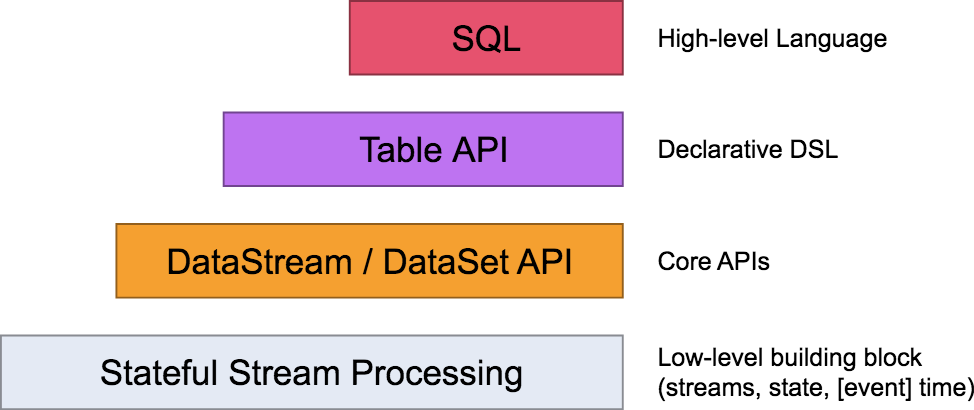
Table API and SQL are at the top. They are advanced API operations provided by Flink. Flink SQL is a development language designed by Flink real-time computing to simplify the computing model and reduce the threshold for users to use real-time computing.
As we mentioned in lesson 04, Flink provides two sets of API s for DataStream and DataSet in the programming model, but it does not achieve the unity of batch flow in fact, because users and developers still develop two sets of code. Because of the addition of Flink table & SQL, it can be said that Flink has achieved the integration of batch flow in fact to some extent.
principle
You may have known Hive before. In the offline computing scenario, Hive almost carries half of the offline data processing. Apache compute is used in its underlying SQL parsing, and Flink also hands over SQL parsing, optimization and execution to compute.
The following figure is a classic schematic diagram of Flink table & SQL implementation. You can see that calculate is in the absolute core position in the whole architecture.
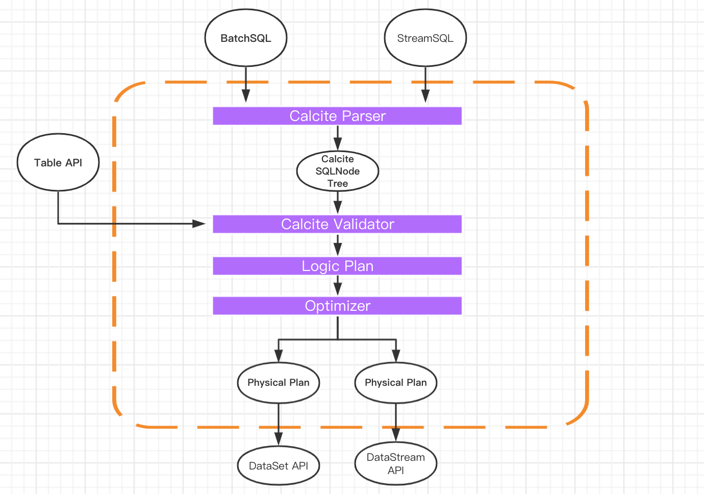
It can be seen from the figure that both batch query SQL and streaming query SQL will be transformed into node tree SQLNode tree through the corresponding converter Parser, and then a logical execution plan will be generated. After optimization, the logical execution plan will generate a real executable physical execution plan and submit it to the API of DataSet or DataStream for execution.
Here, we will not over expand the principle of calculate. Those interested can learn directly on the official website. A complete Flink table & SQL job is also composed of Source, Transformation and Sink:
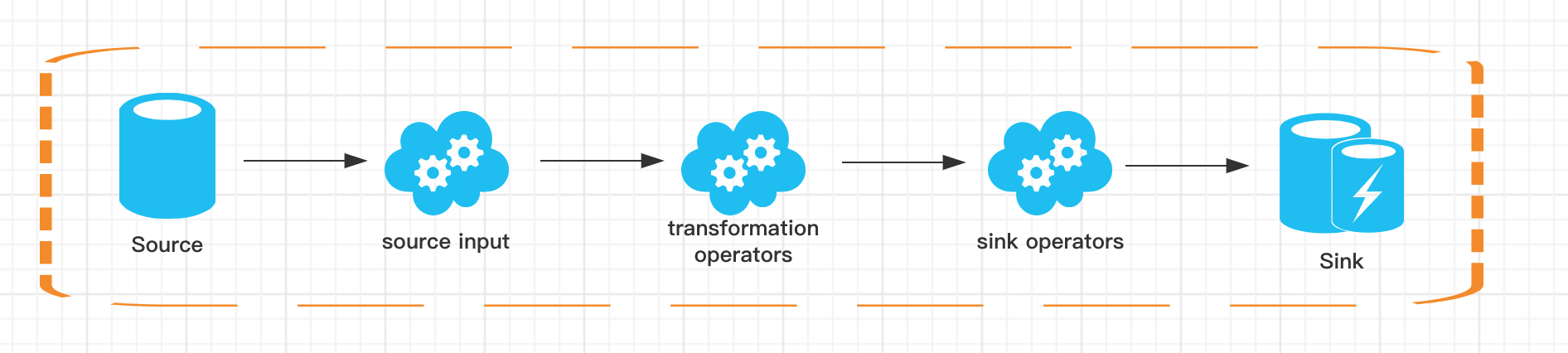
- The Source part comes from external data sources. We often use Kafka, MySQL, etc;
- The Transformation part is the common SQL operators supported by Flink table & SQL, such as simple Select, Groupby, etc. of course, there are more complex multi flow Join, flow and dimension table Join, etc;
- The Sink part refers to the result storage, such as MySQL, HBase or Kakfa.
Dynamic table
Compared with the traditional table SQL query, Flink table & SQL will always be in dynamic data changes when processing stream data, so it has a concept of dynamic table. The query of dynamic table is the same as that of static table. However, when querying dynamic table, SQL will make continuous query and will not terminate.
Let's take a simple example. Flink program accepts a Kafka stream as input. Kafka is the user's purchase record:
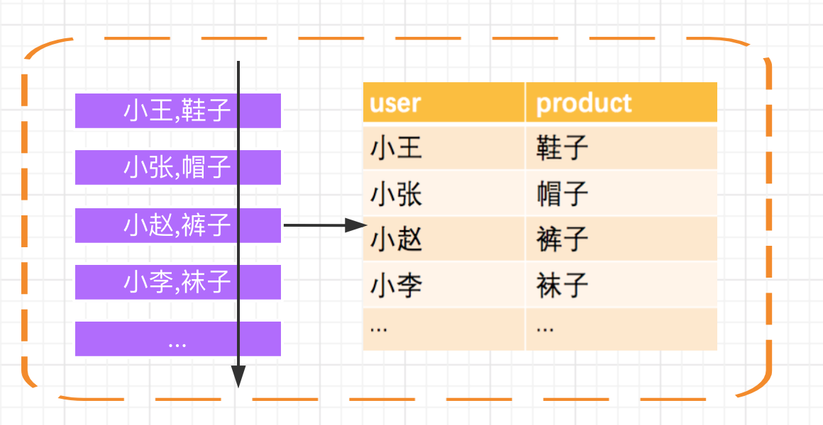
First, Kafka's messages will be continuously parsed into a growing dynamic table, and the SQL we execute on the dynamic table will continue to generate new dynamic tables as the result table.
Flink table & SQL operators and built-in functions
Before we explain the common operators supported by Flink table & SQL, we need to note that since version 0.9, Flink has been in perfect development and iteration. We can also see such tips on the official website:
Please note that the Table API and SQL are not yet feature complete and are being actively developed. Not all operations are supported by every combination of [Table API, SQL] and [stream, batch] input.
The development of Flink table & SQL has been in progress and does not support the calculation logic in all scenarios. From my personal practice point of view, when using the native Flink table & SQL, be sure to query the support of the current version of the official website for table & SQL, and try to choose a scene with clear scene and not extremely complex logic.
Common operators
Currently, Flink SQL supports the following syntax:
query:
  values
  | {
      select
      | selectWithoutFrom
      | query UNION [ ALL ] query
      | query EXCEPT query
      | query INTERSECT query
    }
    [ ORDER BY orderItem [, orderItem ]* ]
    [ LIMIT { count | ALL } ]
    [ OFFSET start { ROW | ROWS } ]
    [ FETCH { FIRST | NEXT } [ count ] { ROW | ROWS } ONLY]

orderItem:
  expression [ ASC | DESC ]

select:
  SELECT [ ALL | DISTINCT ]
  { * | projectItem [, projectItem ]* }
  FROM tableExpression
  [ WHERE booleanExpression ]
  [ GROUP BY { groupItem [, groupItem ]* } ]
  [ HAVING booleanExpression ]
  [ WINDOW windowName AS windowSpec [, windowName AS windowSpec ]* ]

selectWithoutFrom:
  SELECT [ ALL | DISTINCT ]
  { * | projectItem [, projectItem ]* }

projectItem:
  expression [ [ AS ] columnAlias ]
  | tableAlias . *

tableExpression:
  tableReference [, tableReference ]*
  | tableExpression [ NATURAL ] [ LEFT | RIGHT | FULL ] JOIN tableExpression [ joinCondition ]

joinCondition:
  ON booleanExpression
  | USING '(' column [, column ]* ')'

tableReference:
  tablePrimary
  [ matchRecognize ]
  [ [ AS ] alias [ '(' columnAlias [, columnAlias ]* ')' ] ]

tablePrimary:
  [ TABLE ] [ [ catalogName . ] schemaName . ] tableName
  | LATERAL TABLE '(' functionName '(' expression [, expression ]* ')' ')'
  | UNNEST '(' expression ')'

values:
  VALUES expression [, expression ]*

groupItem:
  expression
  | '(' ')'
  | '(' expression [, expression ]* ')'
  | CUBE '(' expression [, expression ]* ')'
  | ROLLUP '(' expression [, expression ]* ')'
  | GROUPING SETS '(' groupItem [, groupItem ]* ')'

windowRef:
    windowName
  | windowSpec

windowSpec:
    [ windowName ]
    '('
    [ ORDER BY orderItem [, orderItem ]* ]
    [ PARTITION BY expression [, expression ]* ]
    [
        RANGE numericOrIntervalExpression {PRECEDING}
      | ROWS numericExpression {PRECEDING}
    ]
    ')'
...
It can be seen that like traditional SQL, Flink SQL supports scenarios including query, connection and aggregation, as well as scenarios including window and sorting. Now I will explain in detail the most commonly used operators.
SELECT/AS/WHERE
Like traditional SQL, SELECT and WHERE are used to filter and filter data. They are applicable to DataStream and DataSet at the same time.
SELECT * FROM Table;
SELECT name,age FROM Table;
Of course, we can also use the combination of =, <, >, < >, > =, < =, AND, OR AND other expressions in the WHERE condition:
SELECT name,age FROM Table where name LIKE '%Xiao Ming%';
SELECT * FROM Table WHERE age = 20;
SELECT name, age
FROM Table
WHERE name IN (SELECT name FROM Table2)
GROUP BY / DISTINCT/HAVING
GROUP BY is used for grouping and DISTINCT is used for de duplication of results. HAVING, like traditional SQL, can be used to filter after aggregate functions.
SELECT DISTINCT name FROM Table;
SELECT name, SUM(score) as TotalScore FROM Table GROUP BY name;
SELECT name, SUM(score) as TotalScore FROM Table GROUP BY name HAVING
SUM(score) > 300;
JOIN
JOIN can be used to combine the data from two tables to form a result table. At present, Flink's JOIN only supports equivalent connection. The JOIN types supported by Flink include:
JOIN - INNER JOIN
LEFT JOIN - LEFT OUTER JOIN
RIGHT JOIN - RIGHT OUTER JOIN
FULL JOIN - FULL OUTER JOIN
For example, associate with user table and product table:
SELECT *
FROM User LEFT JOIN Product ON User.name = Product.buyer

SELECT *
FROM User RIGHT JOIN Product ON User.name = Product.buyer

SELECT *
FROM User FULL OUTER JOIN Product ON User.name = Product.buyer
The meanings of LEFT JOIN, RIGHT JOIN and FULL JOIN are the same as those in our traditional SQL.
WINDOW
According to the different division of window data, there are three types of Apache Flink:
- Scroll the window, the window data has a fixed size, and the data in the window will not be superimposed;
- Sliding window, the window data has fixed size and generation interval;
- Session window: the window data has no fixed size. It is divided according to the parameters passed in by the user, and the window data has no superposition;
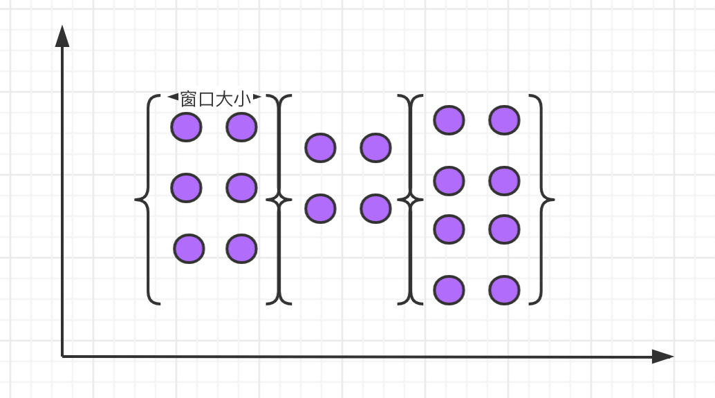
scroll window
The features of the scrolling window are: it has a fixed size and the data in the window will not overlap, as shown in the following figure:
Syntax for scrolling windows:
SELECT
    [gk],
    [TUMBLE_START(timeCol, size)],
    [TUMBLE_END(timeCol, size)],
    agg1(col1),
    ...
    aggn(colN)
FROM Tab1
GROUP BY [gk], TUMBLE(timeCol, size)
For example, we need to calculate the daily order quantity of each user:
SELECT user, TUMBLE_START(timeLine, INTERVAL '1' DAY) as winStart, SUM(amount) FROM Orders GROUP BY TUMBLE(timeLine, INTERVAL '1' DAY), user;
Among them, TUMBLE_START and TUMBLE_END represents the start time and end time of the window, timeLine in toggle (timeLine, INTERVAL '1' DAY) represents the column where the time field is located, and INTERVAL '1' DAY indicates that the time interval is one day.
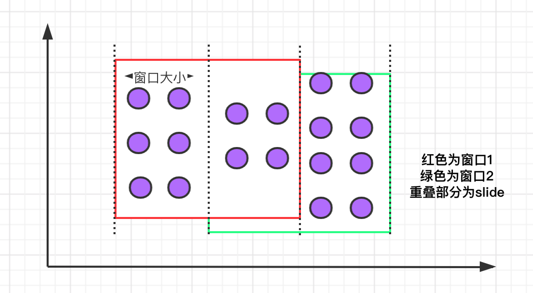
sliding window
The sliding window has a fixed size. Different from the rolling window, the sliding window can control the creation frequency of the sliding window through the slide parameter. It should be noted that data overlap may occur in multiple sliding windows. The specific semantics are as follows:
Compared with scrolling window, the syntax of sliding window has only one more slide parameter:
Copy code
SELECT
    [gk],
    [HOP_START(timeCol, slide, size)] ,
    [HOP_END(timeCol, slide, size)],
    agg1(col1),
    ...
    aggN(colN)
FROM Tab1
GROUP BY [gk], HOP(timeCol, slide, size)
For example, we need to calculate the sales volume of each commodity in the past 24 hours every hour:
Copy code
SELECT product, SUM(amount) FROM Orders GROUP BY HOP(rowtime, INTERVAL '1' HOUR, INTERVAL '1' DAY), product
The INTERVAL '1' HOUR in the above case represents the time interval generated by the sliding window.
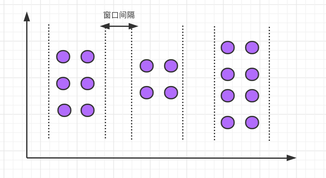
Session window
The session window defines an inactive time. If there are no events or messages within the specified time interval, the session window will be closed.
The syntax of the session window is as follows:
SELECT
    [gk],
    SESSION_START(timeCol, gap) AS winStart,
    SESSION_END(timeCol, gap) AS winEnd,
    agg1(col1),
     ...
    aggn(colN)
FROM Tab1
GROUP BY [gk], SESSION(timeCol, gap)
For example, we need to calculate the order volume of each user in the past 1 hour:
SELECT user, SESSION_START(rowtime, INTERVAL '1' HOUR) AS sStart, SESSION_ROWTIME(rowtime, INTERVAL '1' HOUR) AS sEnd, SUM(amount) FROM Orders GROUP BY SESSION(rowtime, INTERVAL '1' HOUR), user
Built in function
Flink also has a large number of built-in functions, which we can use directly. The built-in functions are classified as follows:
- Comparison function
- Logic function
- Arithmetic function
- String handler
- Time function
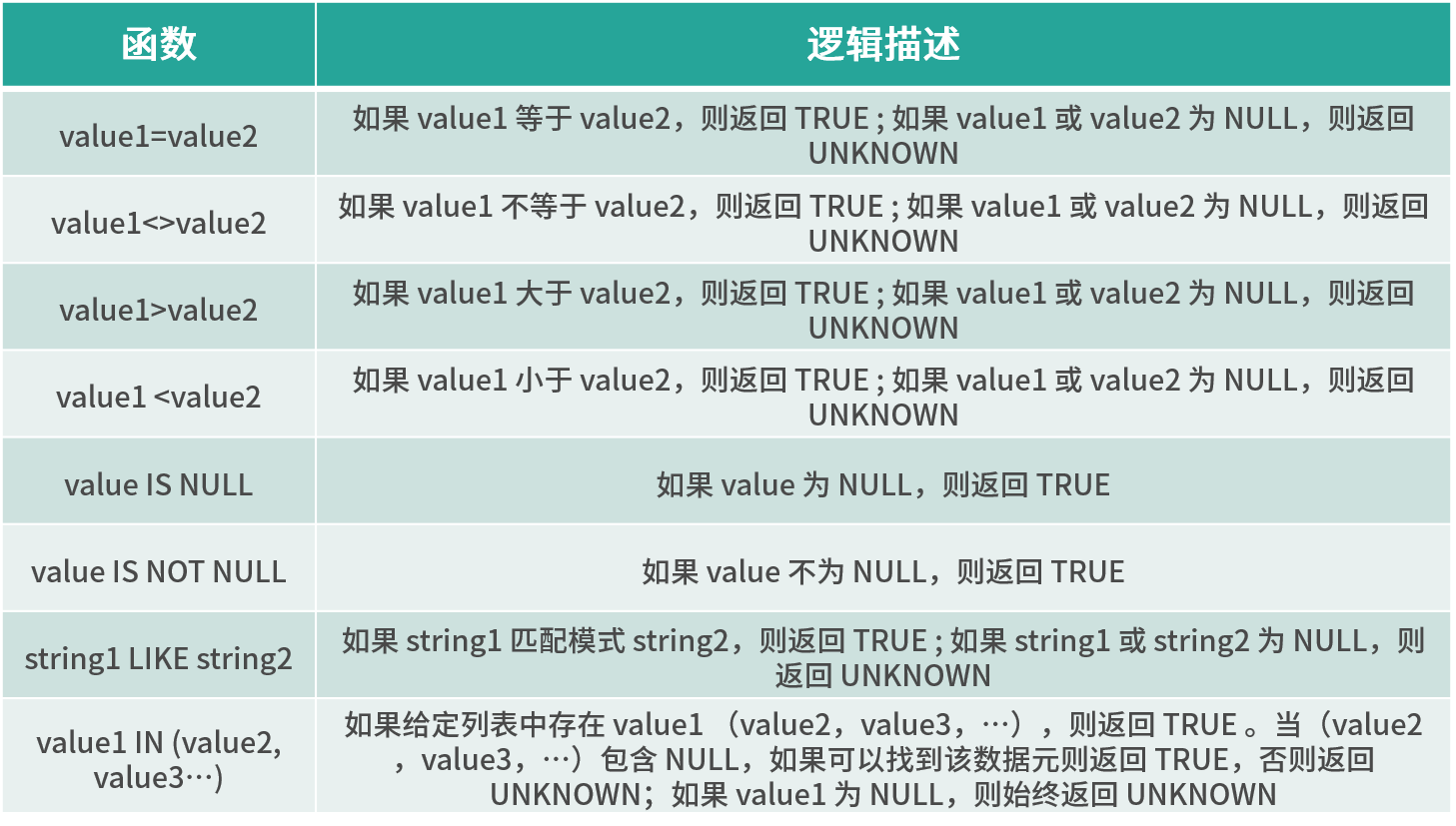
Comparison function
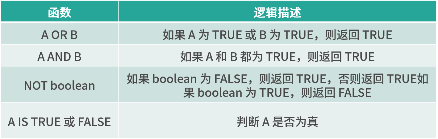
Logic function
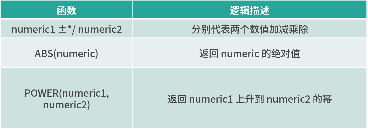
Arithmetic function
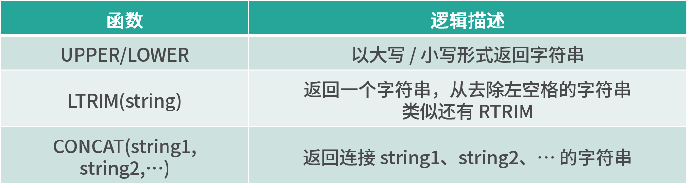
String handler
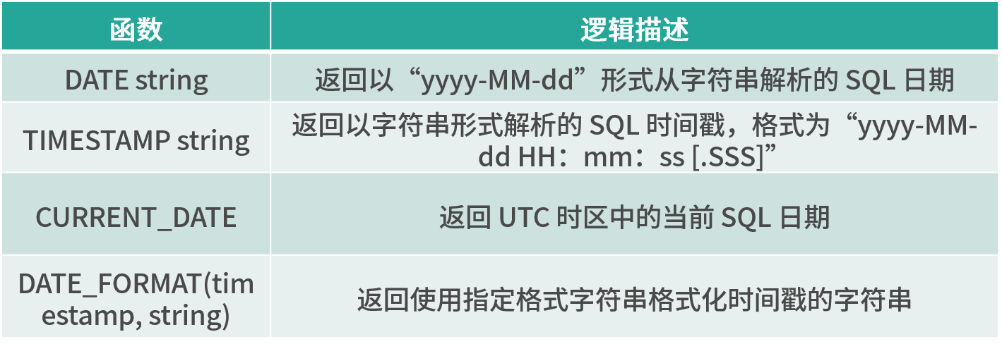
Time function
Flink table & SQL case
The above introduces the principle and supported operators of Flink table & SQL respectively. We simulate a real-time data flow, and then explain the usage of SQL JOIN.
In the last lesson, we used the custom Source function provided by Flink to realize a custom real-time data Source. The specific implementation is as follows:
Copy code
public  class MyStreamingSource implements SourceFunction<Item> {
    private boolean isRunning = true;
    /**
     * Rewrite the run method to produce a continuous source of data transmission
     *
     * @param ctx
     * @throws Exception
     */
    @Override
    public void run(SourceContext<Item> ctx) throws Exception {
        while (isRunning) {
            Item item = generateItem();
            ctx.collect(item);

            //One piece of data per second
            Thread.sleep(1000);
        }
    }

    @Override
    public void cancel() {
        isRunning = false;
    }

    //Randomly generate a piece of commodity data
    private Item generateItem() {
        int i = new Random().nextInt(100);
        ArrayList<String> list = new ArrayList();
        list.add("HAT");
        list.add("TIE");
        list.add("SHOE");
        Item item = new Item();
        item.setName(list.get(new Random().nextInt(3)));
        item.setId(i);
        return item;
    }
}
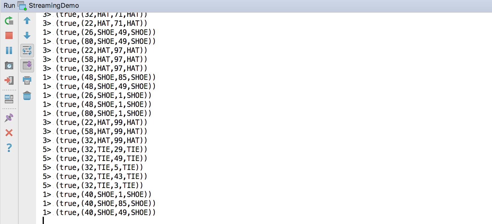
We divide the real-time commodity data stream into two streams, even and odd, for JOIN, provided that the names are the same. Finally, we output the JOIN results of the two streams.
public class JoinDemo extends StreamJavaJob {
    public static void main(String[] args) throws Exception {
        initStreamJob(null, true);

        SingleOutputStreamOperator<Item> source = env.addSource(new MyStreamingSource()).map(new MapFunction<Item, Item>() {
            @Override
            public Item map(Item item) throws Exception {
                return item;
            }
        });

        DataStream<Item> evenSelect = source.split(new OutputSelector<Item>() {
            @Override
            public Iterable<String> select(Item value) {
                List<String> output = new ArrayList<>();
                if (value.getId() % 2 == 0) {
                    output.add("even");
                } else {
                    output.add("odd");
                }
                return output;
            }
        }).select("even");

        DataStream<Item> oddSelect = source.split(new OutputSelector<Item>() {
            @Override
            public Iterable<String> select(Item value) {
                List<String> output = new ArrayList<>();
                if (value.getId() % 2 == 0) {
                    output.add("even");
                } else {
                    output.add("odd");
                }
                return output;
            }
        }).select("odd");


        stEnv.createTemporaryView("evenTable", evenSelect, "name,id");
        stEnv.createTemporaryView("oddTable", oddSelect, "name,id");

        Table queryTable = stEnv.sqlQuery("select a.id,a.name,b.id,b.name from evenTable as a join oddTable as b on a.name = b.name");

        queryTable.printSchema();

        stEnv.toRetractStream(queryTable, TypeInformation.of(new TypeHint<Tuple4<Integer,String,Integer,String>>(){})).print();
        startStreaming();
    }
}
Right click directly to run, and you can see the output on the console:
summary
In this class, we explained the background and principle of Flink table & SQL and the concept of dynamic table; At the same time, it explains the common SQL and built-in functions supported by Flink; Finally, a case is used to explain the use of Flink table & SQL.
Pay attention to the official account: big data technology, reply to information, receive 1024G information.