catalogue
LightGBM parallel optimization
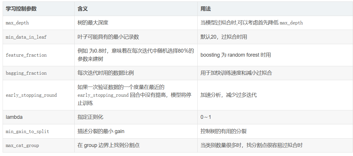
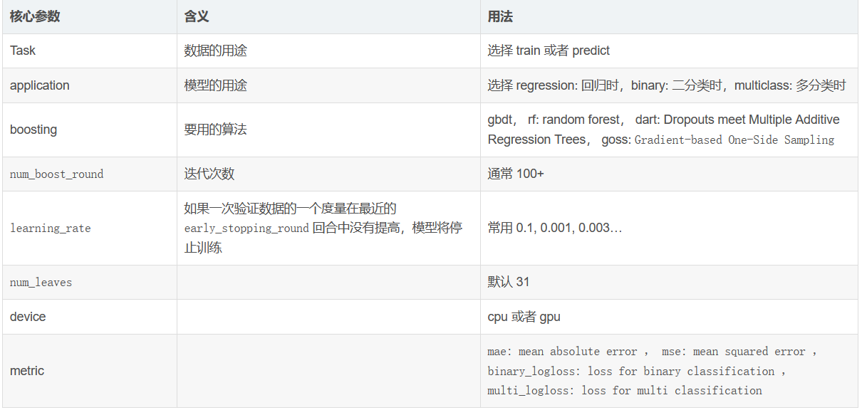
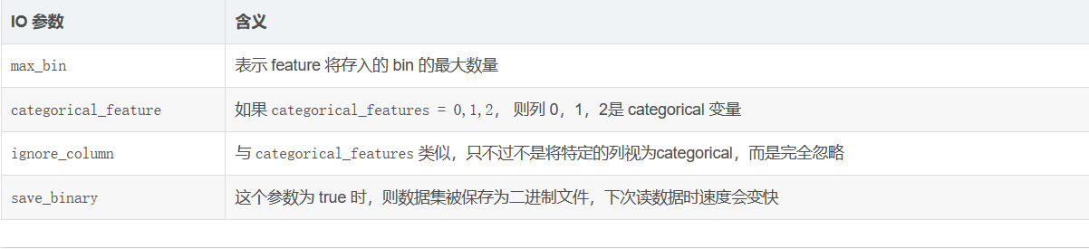
Detailed explanation of parameters
Optimal model and parameters (dataset 1000)
Walk into LightGBM
What is LightGBM?
In the last article, I introduced XGBoost algorithm, which is a big killer in many competitions, but in the process of use, its training takes a long time and occupies a large amount of memory.
In January 2017, Microsoft opened LightGBM on GitHub. Without reducing the accuracy, the speed of the algorithm is increased by about 10 times and the occupied memory is reduced by about 3 times. LightGBM is a fast, distributed and high-performance gradient lifting algorithm based on decision tree algorithm. It can be used in sorting, classification, regression and many other machine learning tasks.
GBDT (Gradient Boosting Decision Tree) is an enduring model in machine learning. Its main idea is to use the iterative training of weak classifier (decision tree) to obtain the optimal model. The model has the advantages of good training effect and difficult over fitting. GBDT is not only widely used in industry, but also usually used in multi classification, click through rate prediction, search sorting and other tasks; It is also a deadly weapon in various data mining competitions. According to statistics, more than half of the champion schemes in Kaggle competitions are based on GBDT.
LightGBM (Light Gradient Boosting Machine) is a framework to realize GBDT algorithm. It supports efficient parallel training, and has the advantages of faster training speed, lower memory consumption, better accuracy, distributed support and rapid processing of massive data.
LightGBM is a gradient lifting framework that uses a tree based learning algorithm.
Common machine learning algorithms, such as neural networks, can be trained in the form of mini batch, and the size of training data will not be limited by memory. In each iteration, GBDT needs to traverse the whole training data many times. If the whole training data is loaded into the memory, the size of the training data will be limited; If it is not loaded into memory, it will consume a lot of time to read and write training data repeatedly. Especially in the face of industrial massive data, the ordinary GBDT algorithm can not meet its needs.
The main reason for LightGBM is to solve the problems encountered by GBDT in massive data, so that GBDT can be better and faster used in industrial practice.
Disadvantages of XGBoost
Before LightGBM was proposed, the most famous GBDT tool was XGBoost, which is a decision tree algorithm based on pre sorting method. The basic idea of this algorithm is: first, all features are pre sorted according to the value of the feature. Secondly, when traversing the segmentation points, use the cost of O(#data) to find the best segmentation point on the feature. Finally, after finding the best segmentation point of a feature, the data is divided into left and right sub nodes.
The advantage of this pre sorting algorithm is that it can accurately find the segmentation points. But the disadvantages are also obvious: first, the space consumption is large. Such an algorithm needs to save the eigenvalues of the data and the results of feature sorting (for example, in order to quickly calculate the segmentation points later, the sorted index is saved), which needs to consume twice the memory of the training data. Each traversal point requires a large cost of computation. Secondly, it also costs a large cost of computation. Finally, it is not friendly to cache optimization. After pre sorting, the access of features to the gradient is a random access, and the access order of different features is different, so the cache cannot be optimized. At the same time, in each layer of long tree, it is necessary to randomly access an array from row index to leaf index, and the access order of different features is also different, which will also cause large cache miss.
Optimization of LightGBM
In order to avoid the defects of XGBoost and speed up the training speed of GBDT model without damaging the accuracy, lightGBM optimizes the traditional GBDT algorithm as follows:
- Decision tree algorithm based on Histogram.
- Unilateral gradient based one side sampling (GOSS): using GOSS can reduce a large number of data instances with only small gradients. In this way, only the remaining data with high gradients can be used when calculating the information gain. Compared with XGBoost, traversing all eigenvalues saves a lot of time and space.
- Mutually Exclusive Feature Bundling(EFB): using EFB, you can bind many mutually exclusive features into one feature, so as to achieve the purpose of dimension reduction.
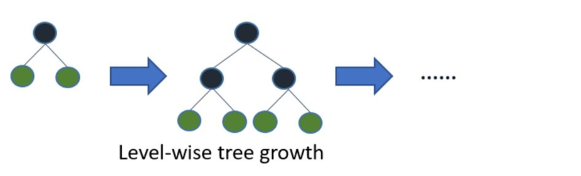
- Leaf wise leaf growth strategy with depth constraints: most GBDT tools use the inefficient level wise decision tree growth strategy, because it treats the leaves of the same layer indiscriminately, which brings a lot of unnecessary overhead. In fact, the splitting gain of many leaves is low, so there is no need to search and split. LightGBM uses a leaf wise algorithm with depth constraints.
- Directly support category feature
- Support efficient parallelism
- Cache hit rate optimization
Basic principles of LightGBM
The growth mode of LightGBM tree is vertical, and other algorithms are horizontal, that is, Light GBM grows the leaves of the tree, and other algorithms grow the hierarchy of the tree.
LightGBM selects the leaves with the largest error to grow. When growing the same leaves, the leaf growing algorithm can reduce more loss than the layer based algorithm.
The following figure explains the implementation of LightGBM and other lifting algorithms
Based on Histogram algorithm, LightGBM is further optimized. Firstly, it abandons the level wise decision tree growth strategy used by most GBDT tools and uses the leaf wise algorithm with depth constraints. The level wise data can split the leaves of the same layer at the same time. It is easy to carry out multi-threaded optimization and control the complexity of the model. It is not easy to over fit. But in fact, level wise is an inefficient algorithm, because it treats the leaves of the same layer indiscriminately, which brings a lot of unnecessary overhead. In fact, the splitting gain of many leaves is low, so there is no need to search and split.
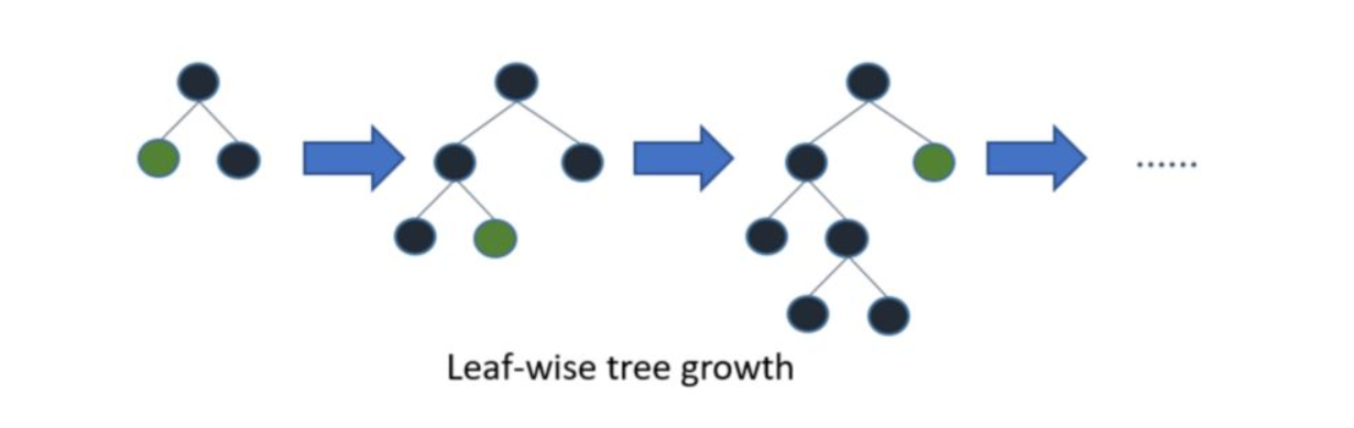
Leaf wise is a more efficient strategy. Each time, find the leaf with the largest splitting gain from all the current leaves, then split and cycle. Therefore, compared with level wise, under the same splitting times, leaf wise can reduce more errors and obtain better accuracy. The disadvantage of leaf wise is that it may grow a deep decision tree and produce over fitting. Therefore, LightGBM adds a maximum depth limit on leaf wise to prevent over fitting while ensuring high efficiency.
 The amount of data is increasing every day. It is difficult for traditional data science algorithms to give results quickly. The prefix 'Light' of LightGBM indicates fast speed. LightGBM can process a large amount of data and occupy little memory at runtime. Another reason why LightGBM is so popular is that it focuses on the accuracy of results. LightGBM also supports GPU learning. Therefore, data scientists widely use LightGBM to deploy data science applications.
Since it can improve the speed, can it be used on small data sets?
may not! LightGBM is not recommended for small datasets. LightGBM is very sensitive to over fitting and is very easy to over fit for small data sets. There is no threshold for how small a data set is, but from my experience, I suggest using LightGBM for data above 10000 +. This is also obvious, because XGBoost can be used for small data sets.
The implementation of LightGBM is very simple, and the complex is the debugging of parameters. LightGBM has more than 100 parameters, but don't worry, you don't need to learn everything.
Histogram algorithm
The basic idea of histogram algorithm is to discretize the continuous floating-point eigenvalues into k integers, and construct a histogram with width K. When traversing the data, the statistics are accumulated in the histogram according to the discrete value as the index. After traversing the data once, the histogram accumulates the required statistics, and then traverses to find the optimal segmentation point according to the discrete value of the histogram.
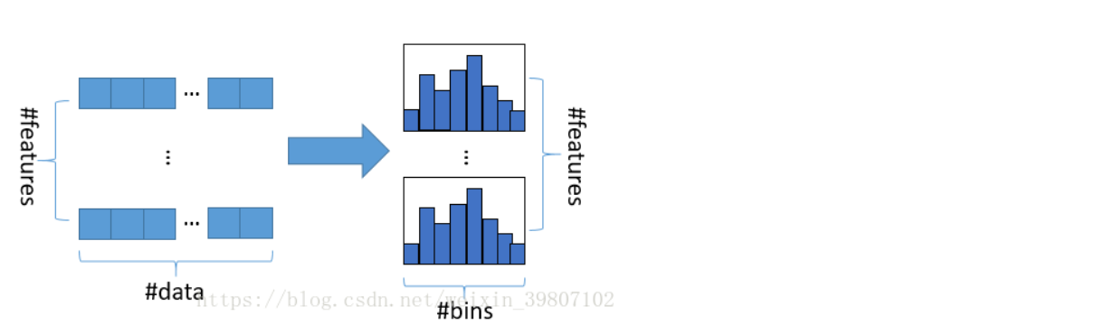
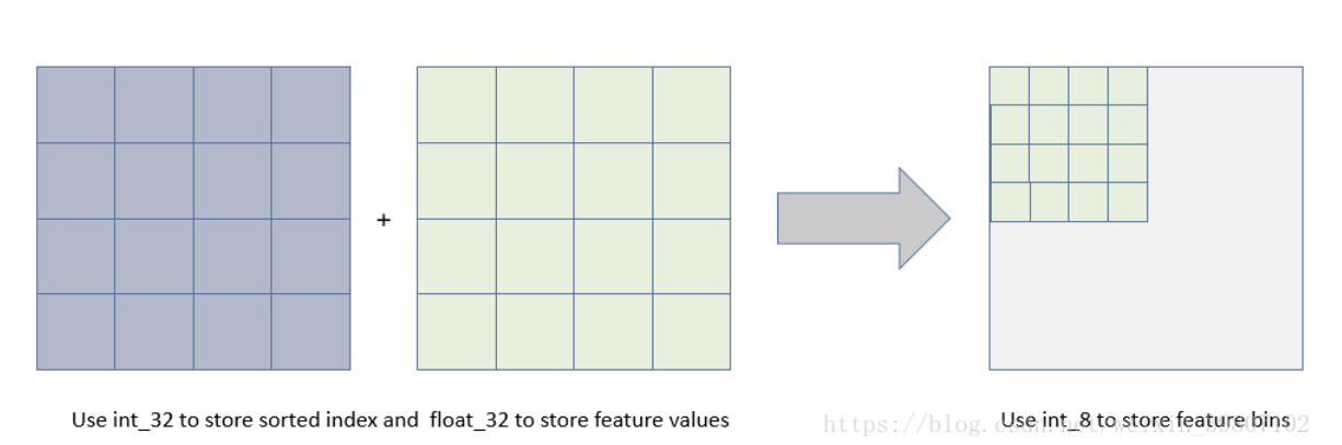
Using histogram algorithm has many advantages. First of all, the most obvious is the reduction of memory consumption. The histogram algorithm not only does not need to store the pre sorted results, but also can only save the value after feature discretization. Generally, 8-bit integer storage is enough for this value, and the memory consumption can be reduced to 1 / 8 of the original. (low memory consumption)
Then the computational cost is greatly reduced. The pre sorting algorithm needs to calculate the split gain every time it traverses an eigenvalue, while the histogram algorithm only needs to calculate K times (K can be considered as a constant), and the time complexity is optimized from O(#data*#feature) to O(k*#features).
Of course, the Histogram algorithm is not perfect. After the feature is discretized, the exact segmentation points are not found, so it will affect the results. However, the results on different data sets show that the discrete segmentation points do not have a great impact on the final accuracy, and sometimes even better.
Histogram acceleration
Another optimization of LightGBM is Histogram difference acceleration. An easily observed phenomenon: the Histogram of a leaf can be obtained by the difference between its parent node's Histogram and its brother's Histogram. Generally, to construct a Histogram, you need to traverse all the data on the leaf, but if the Histogram is poor, you only need to traverse k buckets of the Histogram. Using this method, after constructing a leaf Histogram, LightGBM can get its brother leaf Histogram at a very small cost, and the speed can be doubled.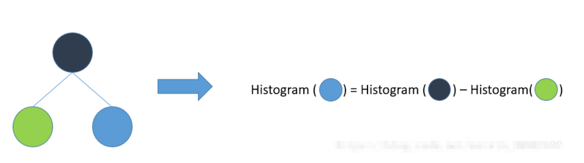
In fact, most machine learning tools cannot directly support category features. Generally, category features need to be transformed into multi-dimensional 0 / 1 features, which reduces the efficiency of space and time. The use of category features is very common in practice. Based on this consideration, LightGBM optimizes the support for category features. Category features can be input directly without additional 0 / 1 expansion. The decision rules of category characteristics are added to the decision tree algorithm. In the experiment on the Expo data set, compared with the 0 / 1 expansion method, the training speed can be accelerated by 8 times, and the accuracy is consistent. To our knowledge, LightGBM is the first GBDT tool to directly support category features.
The stand-alone version of LightGBM has many other detailed optimizations, such as cache access optimization, multithreading optimization, sparse feature optimization and so on. The optimization is summarized as follows:
LightGBM parallel optimization
LightGBM also has the advantage of supporting efficient parallelism. LightGBM natively supports parallel learning. At present, it supports feature parallel and data parallel.
The main idea of feature parallelism is to find the optimal segmentation points on different feature sets of different machines, and then synchronize the optimal segmentation points between machines.
Data parallelism is to let different machines first construct histograms locally, then merge them globally, and finally find the optimal segmentation point on the merged histograms.
LightGBM is optimized for both parallel methods:
In the feature parallel algorithm, the communication of data segmentation results is avoided by saving all data locally;
The amount of communication between different machines is further reduced by combining the histogram and scatter in parallel. Voting based data parallelism further optimizes the communication cost in data parallelism and makes the communication cost constant. When there is a large amount of data, voting parallelism can get a very good acceleration effect.
be careful:
- When the same leaves grow, leaf wise reduces more losses than level wise.
- High speed and efficient processing of big data. It needs lower memory and supports GPU
- Do not use it on a small amount of data. It will be over fitted. It is recommended to use it when there are 10000 + rows of records.
Practice code
Detailed explanation of parameters
The following parameters can improve the accuracy
learning_rate: learning rate
Default: 0.1
Parameter adjustment strategy: it can be set larger at first, such as 0.1. After adjusting other parameters, finally turn down this parameter.
Value range: 0.01 ~ 0.3
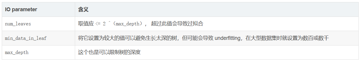
max_depth: tree model depth
Default: - 1
Adjustment strategy: None
Value range: 3-8 (no more than 10)
num_leaves: number of leaf nodes, model complexity

Reduce over fitting
max_bin: number of toolboxes (number of leaf nodes + number of non leaf nodes?)
The maximum number of bin determines the maximum number of groups of features (similar features will be combined)
A small number of bin s will reduce the training accuracy, but may improve the generalization power
LightGBM will be based on max_bin automatically compresses memory. For example, if maxbin=255, LightGBM will use the property value of uint8t
min_data_in_leaf: the minimum amount of data on a leaf Can be used to deal with over fitting
Default: 20
Parameter adjustment strategy: search, try not to be too large.
feature_fraction: the proportion of randomly selected features in each iteration.
Default: 1.0
Parameter adjustment strategy: 0.5-0.9.
Can be used to speed up training
Can be used to deal with over fitting
bagging_fraction: randomly select some data without resampling
Default: 1.0
Parameter adjustment strategy: 0.5-0.9.
Can be used to speed up training
Can be used to deal with over fitting
bagging_freq: the number of bagging. 0 means that bagging is disabled, and a non-zero value means that bagging is executed k times
Default: 0
Parameter adjustment strategy: 3-5
other
lambda_l1:L1 regular
lambda_l2:L2 regular
min_split_gain: the minimum gain of performing segmentation
Default: 0.1
 Code practice
#Import required packages
from sklearn.metrics import precision_score
from sklearn.model_selection import train_test_split
from sklearn.svm import SVC
from sklearn.linear_model import LogisticRegression
from sklearn.ensemble import RandomForestClassifier
import numpy as np
import pandas as pd
import matplotlib.pyplot as plt
from matplotlib.colors import ListedColormap
from sklearn.preprocessing import LabelEncoder
from sklearn.metrics import classification_report#assessment report
from sklearn.model_selection import cross_val_score #Cross validation
from sklearn.model_selection import GridSearchCV #Grid search
import matplotlib.pyplot as plt#visualization
import seaborn as sns#Drawing package
from sklearn.preprocessing import StandardScaler,MinMaxScaler,MaxAbsScaler#Normalization
# Ignore warning
import warnings
warnings.filterwarnings("ignore")
from sklearn.metrics import precision_score
import lightgbm as lgb
Optimal model and parameters (dataset 1000)
Some small partners will have questions. Why our lightGBM effect is not as good as XGBoost? The reason lies in our data, because this is a small data set, and the effect can achieve this. It is entirely the effect of continuously iterating and optimizing parameters.
df=pd.read_csv(r"data.csv")

X=df.iloc[:,:-1]
y=df.iloc[:,-1]
X_train, X_test, y_train, y_test = train_test_split(X,y,test_size=0.2,stratify=y,random_state=1)
model=lgb.LGBMClassifier(n_estimators=39,max_depth=8,num_leaves=12,max_bin=7,min_data_in_leaf=10,bagging_fraction=0.5,
                             feature_fraction=0.59,boosting_type="gbdt",application="binary",min_split_gain=0.15,
                             n_jobs=-1,bagging_freq=30,lambda_l1=1e-05,lambda_l2=1e-05,learning_rate=0.1,
                         random_state=90)
model.fit(X_train,y_train)
# Estimate
y_pred = model.predict(X_test)
'''
Evaluation index
'''
# # Find the same number of predictions as the real one
true = np.sum(y_pred == y_test )
print('The number of predicted results is:', true)
print('The number of mispredicted results is:', y_test.shape[0]-true)
# Evaluation index
from sklearn.metrics import accuracy_score,precision_score,recall_score,f1_score,cohen_kappa_score
print('The accuracy of prediction data is: {:.4}%'.format(accuracy_score(y_test,y_pred)*100))
print('The accuracy of prediction data is:{:.4}%'.format(
      precision_score(y_test,y_pred)*100))
print('The recall rate of predicted data is:{:.4}%'.format(
      recall_score(y_test,y_pred)*100))
# print("F1 value of training data is:", f1score_train)
print('Forecast data F1 The value is:',
      f1_score(y_test,y_pred))
print('Forecast data Cohen's Kappa The coefficient is:',
      cohen_kappa_score(y_test,y_pred))
# Print classification Report
print('The classification report of forecast data is:','\n',
      classification_report(y_test,y_pred))

# ROC curve, AUC
from sklearn.metrics import precision_recall_curve
from sklearn import metrics
# Probability of predicting positive cases
y_pred_prob=model.predict_proba(X_test)[:,1]
# y_pred_prob returns two columns. The first column represents category 0 and the second column represents the probability of category 1
#https://blog.csdn.net/dream6104/article/details/89218239
fpr, tpr, thresholds = metrics.roc_curve(y_test,y_pred_prob, pos_label=2)
#pos_label stands for true positive label, which means it is a good label in the classification. It depends on whether your feature target label is 0,1 or 1,2
roc_auc = metrics.auc(fpr, tpr)  #auc is the area under the Roc curve
# print(roc_auc)
plt.figure(figsize=(8,6))
plt.plot([0, 1], [0, 1], color='navy', lw=2, linestyle='--')
plt.plot(fpr, tpr, 'r',label='AUC = %0.2f'% roc_auc)
plt.legend(loc='lower right')
# plt.plot([0, 1], [0, 1], 'r--')
plt.xlim([0, 1.1])
plt.ylim([0, 1.1])
plt.xlabel('False Positive Rate') #The abscissa is fpr
plt.ylabel('True Positive Rate')  #The ordinate is tpr
plt.title('Receiver operating characteristic example')
plt.show()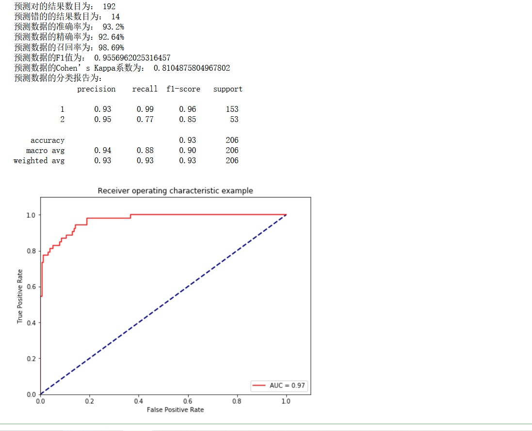
Model tuning
Try to adjust the parameters of the learning curve
To initialize our parameters, we can also determine the approximate parameter position through grid search on the training set, and then use the learning curve to iterate the best parameters
model=lgb.LGBMClassifier(boosting_type='gbdt',objective='binary',metrics='auc',learning_rate=0.01, n_estimators=39, max_depth=4,
                         num_leaves=12,max_bin=15,min_data_in_leaf=11,bagging_fraction=0.8,bagging_freq=20, feature_fraction= 0.7,
lambda_l1=1e-05,lambda_l2=1e-05,min_split_gain=0.5)
For example:
params_test5={'min_split_gain':[0.0,0.1,0.2,0.3,0.4,0.5,0.6,0.7,0.8,0.9,1.0]}

gsearch5 = GridSearchCV(estimator = lgb.LGBMClassifier(boosting_type='gbdt',objective='binary',metrics='auc',learning_rate=0.01,
                                                       n_estimators=1000, max_depth=4, num_leaves=12,max_bin=15,min_data_in_leaf=11,
                                                       bagging_fraction=0.8,bagging_freq=20, feature_fraction= 0.7,
                                                       lambda_l1=1e-05,lambda_l2=1e-05,min_split_gain=0.5),
                                                       param_grid = params_test5, scoring='roc_auc',cv=5)
gsearch5.fit(X_train,y_train)
gsearch5.best_params_, gsearch5.best_score_
learning curve
scorel = []
for i in range(0,200,10):
    model = lgb.LGBMClassifier(n_estimators=i+1,random_state=2022).fit(X_train,y_train)
    score = model.score(X_test,y_test)
    scorel.append(score)

print(max(scorel),(scorel.index(max(scorel))*10)+1)  #The mapping shows that the accuracy changes with the number of estimators, and the neighborhood of 110 is the best
plt.figure(figsize=[20,5])
plt.plot(range(1,200,10),scorel)
plt.show()

## According to the above display, the best point is near 51, and the learning curve is further refined
scorel = []
for i in range(35,45):
    RFC = lgb.LGBMClassifier(n_estimators=i,
                                 n_jobs=-1,
                                 random_state=90).fit(X_train,y_train)
    score = RFC.score(X_test,y_test)
    scorel.append(score)

print(max(scorel),([*range(35,45)][scorel.index(max(scorel))]))  #112 Is the optimal number of estimators #The best score is 0.98945
plt.figure(figsize=[20,5])
plt.plot(range(35,45),scorel)
plt.show()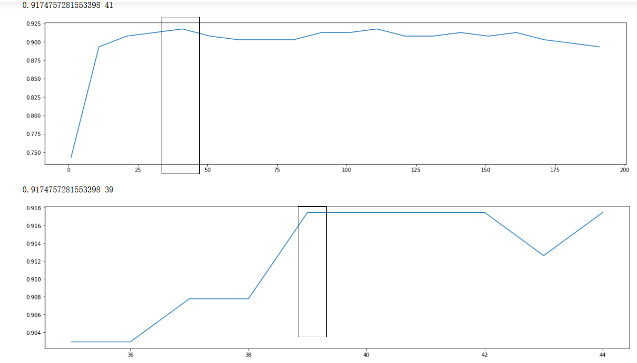
max_depth
scorel = []
for i in range(3,20):
    RFC = lgb.LGBMClassifier(n_estimators=39,max_depth=i,
                                 n_jobs=-1,
                                 random_state=90).fit(X_train,y_train)
    score = RFC.score(X_test,y_test)
    scorel.append(score)

print(max(scorel),([*range(3,20)][scorel.index(max(scorel))]))  #112 Is the optimal number of estimators #The best score is 0.98945
plt.figure(figsize=[20,5])
plt.plot(range(3,20),scorel)
plt.show()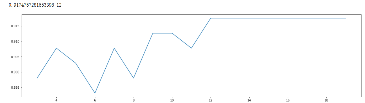
Integer interval parameter tuning (manual modification)
scorel = []
for i in np.arange(7,45,1):
    RFC = lgb.LGBMClassifier(n_estimators=39,max_depth=8,num_leaves=12,max_bin=7,min_data_in_leaf=10,bagging_fraction=0.5,feature_fraction=0.6,
                                 n_jobs=-1,bagging_freq=30,
                                 random_state=90).fit(X_train,y_train)
    score = RFC.score(X_test,y_test)
    scorel.append(score)

print(max(scorel),([*np.arange(7,45,1)][scorel.index(max(scorel))]))  #112 Is the optimal number of estimators #The best score is 0.98945
plt.figure(figsize=[20,5])
plt.plot(np.arange(7,45,1),scorel)
plt.show()
# num_leaves=12,max_bin=15,min_data_in_leaf=11,bagging_fraction=0.8,bagging_freq=20, feature_fraction= 0.7,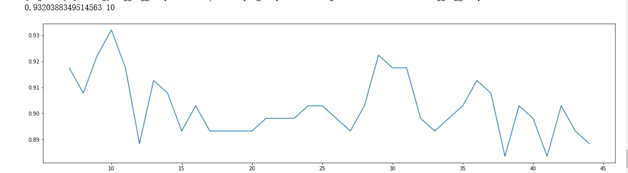
Floating point number parameters (manual modification)
scorel = []
for i in np.arange(0.01,1,0.01):
    RFC = lgb.LGBMClassifier(n_estimators=39,max_depth=8,num_leaves=12,max_bin=7,min_data_in_leaf=10,bagging_fraction=0.5,
                             feature_fraction=0.59,min_split_gain=i,
                             n_jobs=-1,bagging_freq=30,
                             random_state=90).fit(X_train,y_train)
    score = RFC.score(X_test,y_test)
    scorel.append(score)

print(max(scorel),([*np.arange(0.01,1,0.01)][scorel.index(max(scorel))]))  #112 Is the optimal number of estimators #The best score is 0.98945
plt.figure(figsize=[20,5])
plt.plot(np.arange(0.01,1,0.01),scorel)
plt.show()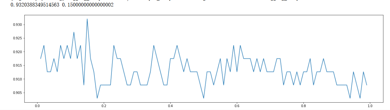
Write to the end:
The scenario used by the algorithm must remember that in the case of large amount of data
Every word
Refuel every day!