catalog:

1, Linear model concept

2, Intuitive principle of LR algorithm

3, Python code implementation algorithm

(notice:

1) In the formula, letters are bold to show vectors

2) LR in this article refers to Linear Regression, not Logistic Regression)

1, Linear model concept

1. Linear model

The so-called linear model is an algorithm model that constructs and trains the hypothesis function according to the characteristic attributes of things in the way of linear combination.

2. General formula of linear model

h θ ( x ) = θ T ⋅ x + b h_\theta(x) = \boldsymbol\theta^T·\textbf{x} + b hθ​(x)=θT⋅x+b
= θ 1 ⋅ x 1 + θ 2 ⋅ x 2 + ⋯ + θ n ⋅ x n + b = \theta_1·x_1 + \theta_2·x_2 +\cdots+ \theta_n·x_n + b =θ1​⋅x1​+θ2​⋅x2​+⋯+θn​⋅xn​+b

Many introductory tutorials will also be written h ( x ) = w T ⋅ x + b h(x)= w^T·x + b h(x)=wT⋅x+b

3. Weight parameter

there θ \theta θ perhaps w w w acts as a weight parameter, θ i ⋅ x i \theta_i·x_i θ In i ⋅ xi θ i \theta_i θ i ， indicates the characteristics x i x_i xi) the importance of.

give an example: h θ ( x ) = 0.03 ⋅ x 1 + 0.8 ⋅ x 2 + 0.2 h_\theta(x) = 0.03·x_1 + 0.8·x_2 + 0.2 hθ​(x)=0.03⋅x1​+0.8⋅x2​+0.2

In short, for this hypothetical function, the characteristics of things x 2 x_2 x2 ratio x 1 x_1 x1 is more important and helps to improve the final prediction accuracy of the algorithm model.

2, Intuitive principle of LR algorithm

1. The most classical linear regression algorithm in linear model.

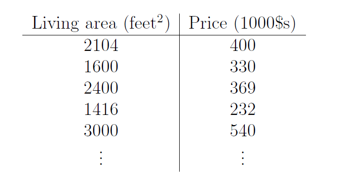
Taking the house price forecast of Ng course as an example, the sample has only one feature x x x: House area. Price is the price of the data sample label y y y.

Put on X o Y XoY On XoY coordinate axis, as shown below:

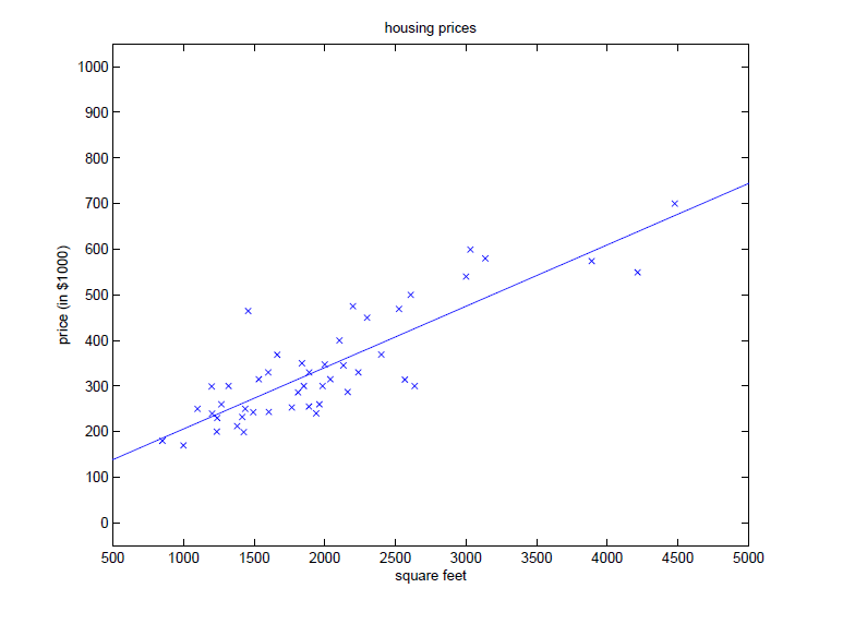
After the data training of the training set, LR algorithm finally learns a hypothesis function, h θ ( x ) = θ T ⋅ x + b h_\theta(x) = \boldsymbol\theta^T·\textbf{x} + b h θ ​(x)= θ T ⋅ x+b is the straight line in the figure. With this function, you can enter the area value of a house arbitrarily to get a predicted price for business reference.

2. The above is the most intuitive principle explanation of LR, which is to get a set of appropriate weight parameters through training. However, there is only the feature of area. In practice, there will be n more features to choose from, which may not be displayed graphically. How to select features involves feature engineering.

3. Algorithm steps

(1) Initialize feature set

First, set the bias term bias, that is, in the hypothetical function b b b. The general practice is to add a column with all eigenvalues of 1 at the beginning (end), as shown in the following example:

b	x 1 x_1 x1​	x 2 x_2 x2​
1	3	10
1	6	11
1	8	10

(2) Initialize parameter set θ \boldsymbol\theta θ

θ = ( θ 0 , θ 1 , θ 2 ) = ( 0 , 0 , 0 ) \boldsymbol\theta = (\theta_0,\theta_1,\theta_2)=(0,0,0) θ=(θ0​,θ1​,θ2​)=(0,0,0)

θ \boldsymbol\theta θ Generally, the initialization is all 0. If the initialization is a random value, it has not been verified whether the convergence speed of the gradient descent algorithm is improved or not

(3) Construct $h_\theta(x) = \theta_0·1 + \theta_1·x_1 + \theta_2·x_2 $

(4) Combine h θ h_\theta h θ And labels y y y. When the gradient descent algorithm is used to converge, a set of feasible parameters are obtained θ ( θ 0 , θ 1 , θ 2 ) \boldsymbol\theta(\theta_0,\theta_1,\theta_2) θ(θ0​,θ1​,θ2​)

3, Python code implementation algorithm

1. Construct feature set and sample label set

def Create_Train_Set(data_set_path):

    #get train_data_set
    train_data = Get_Data_Set(path = data_set_path + 'ds1_train.csv')
    #create train_data label y
    train_data_y = train_data.iloc[:, -1].values.reshape((len(train_data),1))

    #create train_data features and  insert bias into features
    train_data_X = train_data.iloc[:, :-1]
    train_data_X.insert(0,'bias',1)
    train_data_X = train_data_X.values
    
    return train_data_X, train_data_y

2. Construct initialization θ \boldsymbol\theta θ

def Linear_Regression(data_set_path):

    #get train data
    train_data_X, train_data_y = Create_Train_Set(data_set_path)
    #initialize theta 
    theta = np.zeros((train_data_X.shape[1],1))

print(theta)

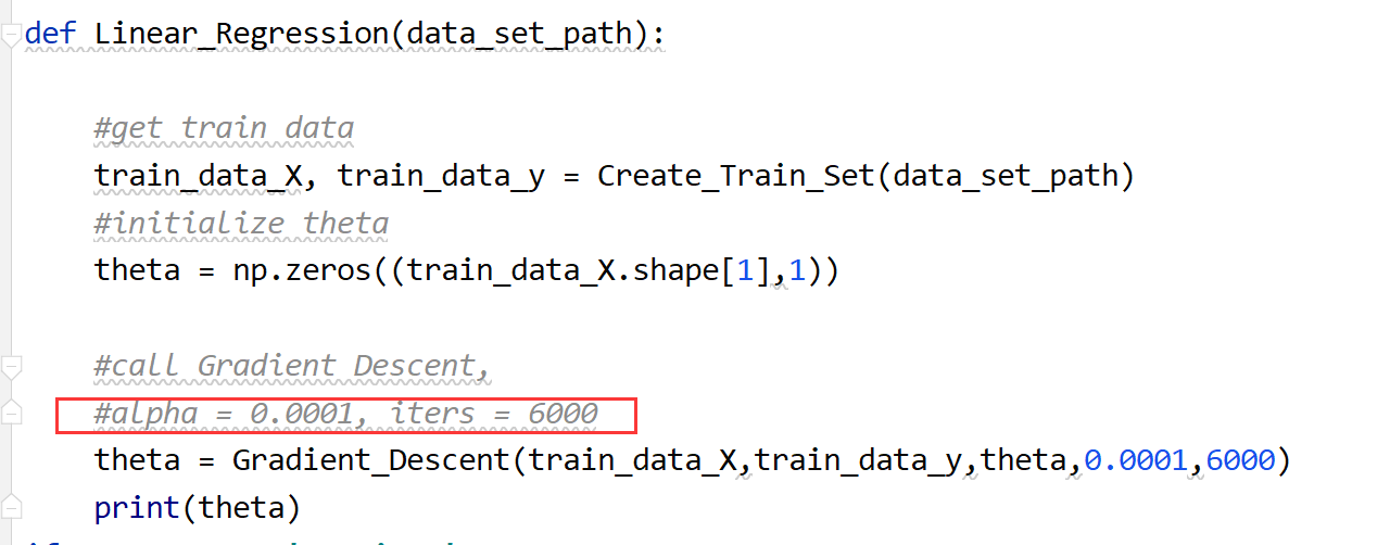
3. Call gradient descent algorithm

According to the principle of gradient descent algorithm, iterative update θ \boldsymbol\theta θ parameter

alpha and iters in the figure below belong to values selected according to subjective wishes, which are adjustment parameters in the general sense

code:

def Gradient_Descent(X,y,theta,alpha, iters):

    for _ in range(iters):
        theta = theta - (X.T @ (X@theta - y) ) * alpha / len(X)

    return theta

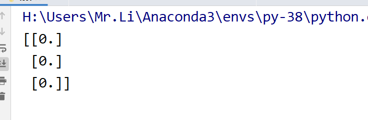
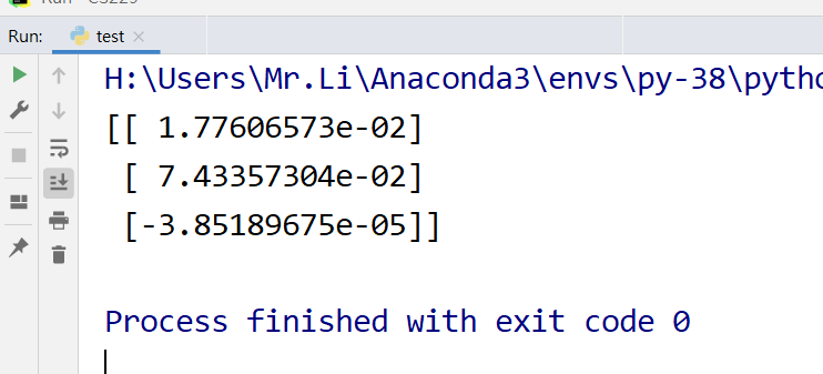
θ \boldsymbol\theta θ Results after 6000 iterations:

4. For LR, the weight parameters are generally obtained θ \boldsymbol\theta θ After, the task is basically completed. The rest is to do feature engineering for the data in the test set and substitute the Hypothesis function to obtain the predicted value

5. Complete code

import pandas as pd
import numpy as np

def Get_Data_Set(path):
    data = pd.read_csv(path)
    return data

def Create_Train_Set(data_set_path):

    #get initial train data
    train_data = Get_Data_Set(path = data_set_path + 'ds1_train.csv')
    #create train_data label y
    train_data_y = train_data.iloc[:, -1].values.reshape((len(train_data),1))

    #create train_data features and  insert bias into features
    train_data_X = train_data.iloc[:, :-1]
    train_data_X.insert(0,'bias',1)
    train_data_X = train_data_X.values

    return train_data_X, train_data_y

def Hypothesis(theta,X):
    """hypothesis function"""
    return X @ theta

def Cost_Function(theta,X,y):
    """cost function"""

    cost = np.power(Hypothesis(theta,X) - y, 2)
    return np.sum(cost) / 2

def Gradient_Descent(X,y,theta,alpha, iters):
    """gradient descent algorithm"""
    for _ in range(iters):
        theta = theta - (X.T @ (X@theta - y) ) * alpha / len(X)

    return theta

def Linear_Regression(data_set_path):

    #get train data
    train_data_X, train_data_y = Create_Train_Set(data_set_path)
    #initialize theta
    theta = np.zeros((train_data_X.shape[1],1))

    #call Gradient Descent,
    #alpha = 0.0001, iters = 6000
    theta = Gradient_Descent(train_data_X,train_data_y,theta,0.0001,6000)


if __name__ == '__main__':
    data_set_path = './data/PS1/'
    Linear_Regression(data_set_path)