Univariate linear regression

Model description

For the model affected by a single variable, we usually abstract it into the form of univariate primary function, and we assume a hypothetical function H( θ)=θ 0+ θ 1x

Cost function

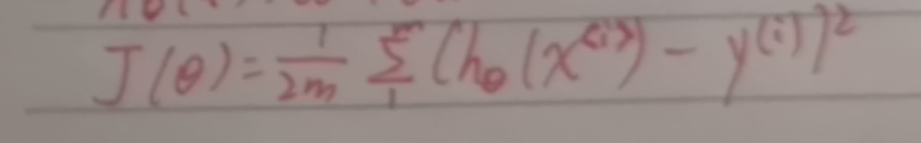
When we make a hypothetical function, we need to determine θ 0 and θ 1 the values of the two coefficients, so that the solved hypothetical function can better fit the data. At this time, we need to introduce the cost function to calculate the difference between the value obtained by the determined function and the value corresponding to the original data.
The specific formula is as follows:

gradient descent

With the cost function, we need to continuously reduce the cost through the cost function to achieve a better solution. At this time, we need to use gradient descent, which is also a method that will be used in many algorithms later.
The specific forms are as follows:

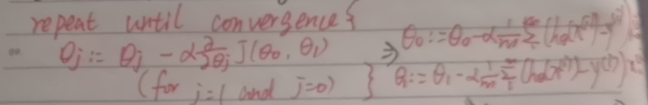
It should be noted here that all data should be calculated first θ The value is being updated.

example

If we assume that the profit of opening a store is linked to the population where it is located, it is obvious that we can assume a univariate linear function to fit it.

'''
Author: csc
Date: 2021-05-02 11:00:18
LastEditTime: 2021-05-03 23:53:47
LastEditors: Please set LastEditors
Description: In User Settings Edit
FilePath: \undefinedd:\pycharm_code\simple_varia\main.py
'''
import numpy as np
import pandas as pd
import matplotlib.pyplot as plt


def costfunction(x, y, theta):
    inner = np.power(x @ theta - y, 2)
    return np.sum(inner) / (2 * len(x))


def gradientDescent(x, y, theta, alpha, iters):
    costs = []

    for i in range(iters):
        theta = theta - (x.T @ (x @ theta - y)) * alpha / len(x)
        cost = costfunction(x, y, theta)
        costs.append(cost)

        if i % 100 == 0:
            print(cost)

    return theta, costs


def main():
    data = pd.read_csv('C:\\Users\\CSC\\Desktop\\hash\\ML_NG\\01-linear regression\\ex1data1.txt',
                       names=['population', 'profit'])

    data.plot.scatter('population', 'profit', label='population')
    data.insert(0, 'ones', 1)

    x = data.iloc[:, 0:-1]
    y = data.iloc[:, -1]
    x = x.values
    y = y.values
    y = y.reshape(x.shape[0], 1)
    theta = np.zeros((x.shape[1], 1))
    
    cost_init = costfunction(x, y, theta)
    print("cost_init is  ", end=' ')
    print(cost_init)

    alpha = 0.01
    iters = 2000
    theta, costs = gradientDescent(x, y, theta, alpha, iters)

    fig, ax = plt.subplots()
    ax.plot(np.arange(iters), costs)
    ax.set(xlabel='iters',
           ylabel='cost',
           title='cost vs iters')
    plt.savefig("cost.png")
    plt.show()

    _x = np.linspace(y.min(), y.max(), 100)
    _y = theta[0, 0] + theta[1, 0] * _x
    fig, ax = plt.subplots()
    ax.scatter(x[:, 1], y, label='training data')
    ax.plot(_x, _y, 'r', label='predict')
    ax.legend()
    ax.set(xlabel='populaiton',
           ylabel='profit')
    plt.savefig("result.png")
    plt.show()


if __name__ == '__main__':
    main()

Multivariate linear regression

Feature scaling & learning rate

When our predicted value is no longer determined by one variable, but by multiple variables, the dimension of each variable needs to be considered at this time. If their data differ too much in the coordinate axis, the gradient will decline slowly and affect the operation efficiency of the algorithm.
X = (x-u) / s usually we use this form for feature scaling, where u is the mean, s can be the maximum or standard deviation.
Ideally, the feature scaling is between [- 1,1], but the actual scaling to [- 3,3] is also acceptable

It has been proved here that the learning rate is small enough, J( θ) Will be small enough

example

Assuming a house is ready to be sold, it is known that the price of the house is affected by the size of the area and the number of bedrooms.

'''
Author: csc
Date: 2021-05-02 18:31:06
LastEditTime: 2021-05-04 10:25:33
LastEditors: Please set LastEditors
Description: In User Settings Edit
FilePath: \undefinedd:\pycharm_code\mul_varia\main.py
'''
import numpy as np
import pandas as pd
import matplotlib.pyplot as plt


def normalize_feature(data):
    return (data - data.mean()) / data.std()


def costfunction(x, y, theta):
    inner = np.power(x @ theta - y, 2)
    return np.sum(inner) / (2 * len(x))


def gradientDescent(x, y, theta, alpha, iters):
    costs = []

    for i in range(iters):
        theta = theta - (x.T @ (x @ theta - y)) * alpha / len(x)
        cost = costfunction(x, y, theta)
        costs.append(cost)

        if i % 100 == 0:
            print(cost)

    return theta, costs


def main():
    data = pd.read_csv('C:\\Users\\CSC\\Desktop\\hash\\ML_NG\\01-linear regression\\ex1data2.txt',
                       names=['size', 'bedrooms', 'price'])
    # normalization
    data = normalize_feature(data)
    # deal data
    data.insert(0, 'ones', 1)
    x = data.iloc[:, 0:-1]
    y = data.iloc[:, -1]
    x = x.values
    y = y.values
    y = y.reshape(x.shape[0], 1)
    # cost
    theta = np.zeros((x.shape[1], 1))
    cost_init = costfunction(x, y, theta)
    print()
    print(cost_init)
    # gradientdecent
    candinate_alpha = [0.0003, 0.003, 0.03, 0.0001, 0.001, 0.01]
    iters = 2000
    fig, ax = plt.subplots()
    for alpha in candinate_alpha:
        _, costs = gradientDescent(x, y, theta, alpha, iters)
        print()
        ax.plot(np.arange(iters), costs, label=alpha)
        ax.legend()

    ax.set(xlabel='iters',
           ylabel='cost',
           title='cost vs iters')
    plt.savefig("alpha.png")
    plt.show()


if __name__ == '__main__':
    main()

Normal equation

concept

In the linear regression equation described above, we use the gradient descent algorithm to solve it iteratively θ， Although it is also applicable to many methods in later learning - strong applicability, it will become very annoying when we have enough variables. So is there a way to solve it directly - normal equation. As proved by mathematicians, the normal equation is as follows:

θ=(XTX)-1XTy

Obviously, we use i the inverse matrix, but we don't need to consider whether it is reversible. Even if it is irreversible, it can still be processed in the packaged function. There are two main reasons for the irreversibility of the matrix: 1. Too many characteristic variables; 2. Redundant characteristic variables

Advantages and disadvantages

However, there are advantages and disadvantages. Although the normal equation is concise and can be solved directly without learning rate and iteration, we note that it performs multiple matrix multiplication operations, and the time complexity of each matrix operation is O(n3), so it can be used when the number of data sets m is tens of thousands or less. For larger data sets, we use the gradient descent method. Due to the characteristics of the gradient descent method, it can still work smoothly when the data set is large

code

import numpy as np
import pandas as pd
import matplotlib.pyplot as plt


def normalEquation(x, y):
    theta = np.linalg.inv(x.T@x)@x.T@y
    return theta


def main():
    data = pd.read_csv('C:\\Users\\CSC\\Desktop\\hash\\ML_NG\\01-linear regression\\ex1data1.txt',
                       names=['population', 'profit'])
    data.insert(0, "ones", 1)
    x = data.iloc[:, 0:-1]
    y = data.iloc[:, -1]
    x = x.values
    y = y.values
    y = y.reshape(x.shape[0], 1)
    theta = normalEquation(x, y)
    print(theta)


if __name__ == '__main__':
    main()