Linear transformation + DFT + filtering

Recently, I opened an article on Fourier transform, which shows how to expand an input signal in time domain into the superposition of multiple sine and cosine signals in the form of animation. It looks like I'm impressed, understand, and then forget.

In fact, when you think about it carefully, Fourier transform becomes the coordinate system. In terms of discrete data, the input signal in time domain is actually a (column) vector in the standard coordinate system x ∈ R N × 1 \mathbf{x} \in \mathbb{R}^{N\times 1} x∈RN × 1. Fourier transform is to change the coordinate system through linear transformation to form a new vector: x ^ = F x \hat{\mathbf{x}} = \mathbf{F}\mathbf{x} x^=Fx.

Let's review the matrix linear transformation first. For details, see the previous article: Matrix in linear algebra.

linear transformation

Suppose we have a vector v = [ 1 ; 2 ] \mathbf{v} = [1; 2] v=[1;2], generally, 1 and 2 represent the projection of the vector on the two axes of the standard coordinate system, which can also be used as a matrix, M \mathbf{M} M. To indicate: M = [ 1 0 0 1 ] \mathbf{M} = \begin{bmatrix}1 & 0\\ 0 & 1\end{bmatrix} M=[10​01​]. If this vector is based on another coordinate system, for example: [ 0 − 1 1 0 ] \begin{bmatrix}0 & -1\\ 1 & 0\end{bmatrix} [01 − 10] (the coordinate system rotates 90 degrees counterclockwise), we can calculate the projection of this vector in the standard coordinate system through the following calculation:
v ′ = [ 0 1 − 1 0 ] v = [ − 2 1 ] \mathbf{v}^{'} = \begin{bmatrix}0 & 1\\ -1 & 0\end{bmatrix}\mathbf{v} = \begin{bmatrix}-2 \\ 1\end{bmatrix} v′=[0−1​10​]v=[−21​]

The meaning of linear transformation is to put a data that is not easy to analyze in the standard coordinate system under another coordinate system, which can often make data analysis particularly simple.

DFT + filtering

Back to the discrete Fourier transform, the standard coordinate system will be transformed into a new coordinate system by the matrix F \mathbf{F} F indicates. Vector in new coordinate system x \mathbf{x} x is projected into the standard coordinate system, and we get x ^ \hat{\mathbf{x}} x^. As for the matrix F \mathbf{F} F. All relevant books have its expression:
[ 1 1 1 ⋯ 1 1 ω n ω n 2 ⋯ ω n n − 1 1 ω n 2 ω n 4 ⋯ ω n 2 ( n − 1 ) ⋮ ⋮ ⋮ ⋱ ⋮ 1 ω n n − 1 ω n 2 ( n − 1 ) ⋯ ω n ( n − 1 ) 2 ] \begin{bmatrix} 1 & 1 & 1 & \cdots & 1\\ 1 & \omega_n & \omega_n^2 & \cdots & \omega_n^{n-1}\\ 1 & \omega_n^2 & \omega_n^4 & \cdots & \omega_n^{2(n-1)}\\ \vdots & \vdots & \vdots & \ddots & \vdots\\ 1 & \omega_n^{n-1} & \omega_n^{2(n-1)} & \cdots & \omega_n^{(n-1)^2} \end{bmatrix} ⎣⎢⎢⎢⎢⎢⎢⎡​111⋮1​1ωn​ωn2​⋮ωnn−1​​1ωn2​ωn4​⋮ωn2(n−1)​​⋯⋯⋯⋱⋯​1ωnn−1​ωn2(n−1)​⋮ωn(n−1)2​​⎦⎥⎥⎥⎥⎥⎥⎤​
Among them, ω n = e − 2 π i / n \omega_n=e^{-2\pi i/n} ω n​=e−2πi/n. As for how to get this from the representation of sine and cosine function through Euler transform ω \omega ω I won't repeat it.

In MATLAB calculation, for example, we randomly generate a length of 50 50 50 time domain signal s \mathbf{s} s. We can specifically express the matrix through the above expression and the known signal length F \mathbf{F} F. Then you can find out s ^ \hat{\mathbf{s}} s ^ has:

s = rand(50, 1);

n = length(s);
w = exp(-1i*2*pi/n);

[I,J] = meshgrid(1:n,1:n);
F = w.^((I-1).*(J-1));

s_h = F*s;

Of course, this calculation method is often time-consuming in practical application, so there is fast Fourier transform! An example using FFT and DFT is given below:

Fs = 96e3;            % Sampling frequency                    
T = 1/Fs;             % Sampling period       
L = 1024;             % Length of signal
t = (0:L-1)*T;        % Time vector

S = 0.7*sin(2*pi*5e3*t) + sin(2*pi*12e3*t) + sin(2*pi*18e3*t) + sin(2*pi*26e3*t);

subplot(3,1,1), plot(Fs*t(1:200), S(1:200))

f = Fs*(0:(L/2))/L;

tic
Y = fft(S);
timeElapsed = toc

P2 = abs(Y/L);
P1 = P2(1:L/2+1);
P1(2:end-1) = 2*P1(2:end-1);

subplot(3,1,2), plot(f,P1)


tic
n = length(S);
w = exp(-1i*2*pi/n);
[I,J] = meshgrid(1:n,1:n);
DFT = w.^((I-1).*(J-1));
Y2 = DFT*S';
timeElapsed = toc

P2 = abs(Y2/L);
P1 = P2(1:L/2+1);
P1(2:end-1) = 2*P1(2:end-1);

subplot(3,1,3), plot(f,P1)

Record the operation time through tic'toc of MATLAB. The time given in my notebook is 0.0032 and 0.1162 seconds, corresponding to FFT and DFT. Notes in the code:

• sampling frequency F s F_s Fs # and sample length L L L determines the resolution of each spectral line. In the above example, the data length obtained after Fourier transform is also the same L L 50. Where the interval between each point is: F s / L = 93.75 F_s/L = 93.75 Fs​/L=93.75 Hz.
• The number of spectrum bars that can be displayed is half of the input length of the selected Fourier transform (sampling law).

Based on this knowledge, we can easily use Fourier transform in practice. For example, we can observe a signal through the FFT function of the oscilloscope. Through the spectrum diagram, we can filter some noise signals by modifying the circuit. If the signal is disturbed by white noise, for example:

Fs = 20e3;            % Sampling frequency                    
T = 1/Fs;             % Sampling period       
L = 1024;             % Length of signal
t = (0:L-1)*T;        % Time vector

S = sin(2*pi*1e3*t) + sin(2*pi*5e3*t);
S_n = S + 2.5*randn(size(t)); % Add some noise

subplot(3,1,1)
plot(Fs*t(1:200), S(1:200),'k','LineWidth',1.2), hold on
plot(Fs*t(1:200), S_n(1:200),'r','LineWidth',1.5)
legend('Clean','Noisy')


f = Fs*(0:(L/2))/L;
Y = fft(S_n);
PSD = Y.*conj(Y)/L; % Power spectrum (power per freq)

%Use the PSD to filter out noise
indices = PSD>100; % Find all freqs with large power
PSDclean = PSD.*indices; % Zero out all others

subplot(3,1,2)
plot(f,PSD(1:L/2+1),'r','LineWidth',1.5), hold on
plot(f,PSDclean(1:L/2+1),'b','LineWidth',1.2)
legend('Noisy','Filtered')

Y = indices.*Y;
S_f = ifft(Y); % Inverse FFT for filtered time signal
subplot(3,1,3)
plot(Fs*t(1:200), S(1:200),'k','LineWidth',1.2), hold on
plot(Fs*t(1:200), S_f(1:200),'b','LineWidth',1.2)
legend('Clean','Filtered')

Run the above code to get the following figure:

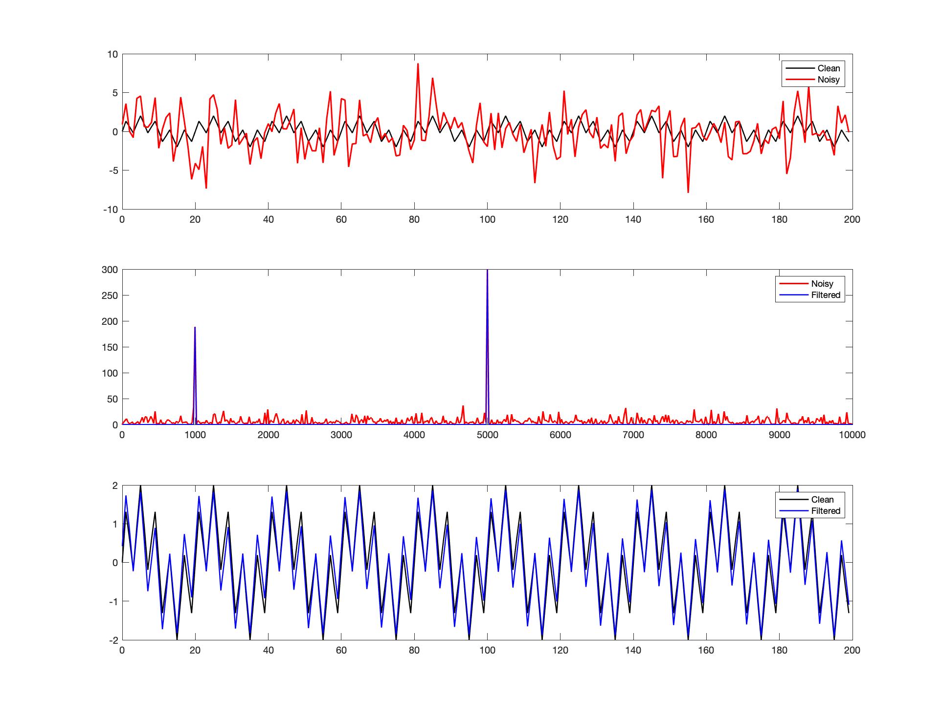
We can see that after adding Gaussian noise, the original signal is chaotic. Through Fourier transform, we can see that except for two frequency points with strong power, the others are very weak signals. We can filter those weak signals by setting a threshold. The signal obtained after inverse transformation is basically consistent with the original signal.