Logistic regression

The basic idea of logistic regression is to find a logical function, map the input characteristics (x1,x2) into (0-1), and then classify them according to whether they are greater than 0.5.

In order to carry out mathematical description, the mapping relation kernel logic function is set; Assuming that the mapping relationship is linear, there are:

  

Namely

At this time, the value of f(x) can be any value, which needs to be remapped (0-1) through the logical function.

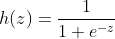
In logistic regression, the logical function is h(z), i.e. sigmoid function:

Draw h(z) on the Z field, and the image is:

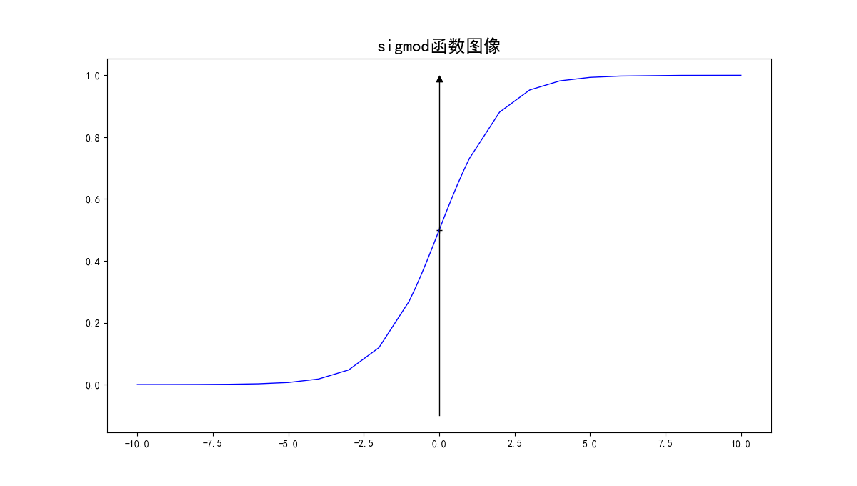
It can be seen that when f (X) > 0, feature X will be classified as class 1, and when f (X) < 0, feature X will be classified as class 0.

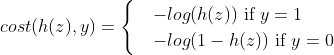
Loss function: the cost loss function should be as small as possible. Therefore, when the real label is 1, the closer h(z) is to 1, the better, then:

The closer to 0; When the real label is 0, the closer h(z) is to 0, the better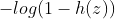The closer to 0; Therefore, the final loss function is defined as:

The above formula can be rewritten as:

With the loss function, the gradient descent method can be used for derivation optimization.

torch

torch is a framework tool specially used to build neural networks, which encapsulates NN Module parent class network structure, variable parameter tensor, variable, NN Bcewithlogitsloss logistic regression loss function optim.SGD gradient descent function and a series of network functions can easily and quickly build a neural network.

1,Variable

It means variable. In essence, it is a variable that can be changed. Different from int variable, it is a variable that can be changed, which just conforms to the attribute of back propagation and parameter update.

Specifically, the Variable in the pytorch is a geographical location where the values will change. The values inside will change constantly, just like a basket containing eggs, and the number of eggs will change constantly. Who is the egg inside? Naturally, it is the tensor in pytorch. (that is, pytorch is calculated by tensor, and the parameters in tensor are in the form of variables). If it is calculated with a Variable, it returns a Variable of the same type. Tensor is a multidimensional matrix.

2,torch.Tensor([1,2])

Generate tensor, [1.0, 2.0], the data in the network must be tensor, and torch Tensor is a function that converts a certain type of value to tensor

3,torch.manual_seed(2)

Set CPU fixed random number and set dimension, torch cuda. manual_ Seed (number) sets a fixed random number for the GPU. After setting, torch When rand (2) is executed, the same random number will be generated every time, which is convenient to observe the improvement and optimization of the model.

For example, chestnuts:

Now, classify the size of numbers into 2. Set the mode category to 1 for numbers greater than 2, and 0 for numbers less than or equal to 2

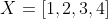
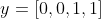
Suppose there are 4 training samples in total, and the samples and labels are as follows:

,     

Then use torch to build your own network and train the code as follows:

import torch
from torch.autograd import Variable

torch.manual_seed(2)
x_data = Variable(torch.Tensor([[1.0], [2.0], [3.0], [4.0]]))
y_data = Variable(torch.Tensor([[0.0], [0.0], [1.0], [1.0]]))

#Define network model
#First create a base class module, all from the parent class torch nn. Module inherits the fixed writing method of pytoch network
class Model(torch.nn.Module):
	def __init__(self):##Fixed writing method, define the constructor, and the parameter is self
		super(Model, self).__init__()  #Inherit parent class, initial parent class or NN Module.__ init__ (self)
		####Define the layers and functions to be used in the class
		self.linear = torch.nn.Linear(1, 1)  #In the linear mapping layer, torch comes with its own package. The input dimension and output dimension are both 1, that is, y=linear(x)==y=wx+b, which will be automatically generated according to
        ####The dimensions of x and y determine the dimensions of W and B.

	def forward(self, x):###Define the forward delivery process diagram of the network
		y_pred = self.linear(x)
		return y_pred

model = Model()  #Network instantiation

#Define loss and optimization methods
criterion = torch.nn.BCEWithLogitsLoss()  #Loss function, encapsulated logical loss function, i.e. cost function
optimizer = torch.optim.SGD(model.parameters(), lr=0.01)   #Optimize gradient descent
#optimizer = torch.optim.SGD(model.parameters(), lr=0.01, weight_decay=0.001)
#Pytorch class method, regularization method, add a weight_ Regularize the decay parameter

#befor training
hour_var = Variable(torch.Tensor([[2.5]]))
y_pred = model(hour_var)####When there is x input, the forward function will be called to directly predict a 2.5 classification
print("predict (before training)given", 4, 'is', float(model(hour_var).data[0][0]>0.5))
########
#####Start training
epochs = 40##Number of iterations
for epoch in range(epochs):
	#Calculate grads and cost
	y_pred = model(x_data)   #x_data Input data into the model####y is the prediction result
	loss = criterion(y_pred, y_data)#####Seek loss
	print('epoch = ', epoch+1, loss.data[0])
	#Back propagation three piece set for fixed use. After defining loss as a loss, it is directly lost Backword updates w and b in the linear map until the classification is correct.
	optimizer.zero_grad() #Gradient clearing
	loss.backward() #Back propagation
	optimizer.step()  #Optimization iteration

#After training
hour_var = Variable(torch.Tensor([[4.0]]))
y_pred = model(hour_var)
print("predict (after training)given", 4, 'is', float(model(hour_var).data[0][0]>0.5))

The operation results are as follows:

predict (before training)given 4 is 0.0
predict (after training)given 4 is 1.0

It can be seen that correct 2 classification can be achieved after training