Logistic Regression model and Python implementation

http://www.cnblogs.com/sumai

1. Model

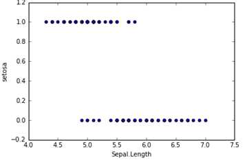
In the classification problem, for example, to judge whether the e-mail is spam and whether the tumor is positive, the target variable is discrete, and there are only two values, usually coded as 0 and 1. Suppose we have a feature X and draw a scatter diagram. The results are as follows. At this time, if we use linear regression to fit a straight line: h θ (X) =  θ 0+ θ 1X, if Y ≥ 0.5, it is judged as 1, otherwise it is 0. In this way, we can also build a model for classification, but there will be many shortcomings, such as poor robustness and low accuracy. Logistic regression is more suitable for such problems.

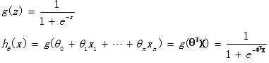
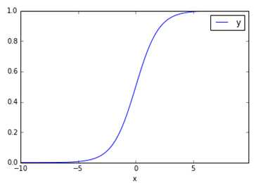
The logistic regression hypothesis function is as follows, which is θ TX makes a function g transformation, which maps to the range from 0 to 1, and function g is called sigmoid function or logistic function. The function image is shown in the figure below. When we enter features, we get h θ (x) In fact, it is the probability value that this sample belongs to the classification of 1. In other words, logistic regression is used to obtain the probability that the sample belongs to a classification.

2. Evaluation

Recall the loss function used in previous linear regression:

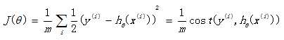
If this loss function is also used in logistic regression, the obtained function J is a non convex function with multiple local minima, which is difficult to solve. Therefore, it is necessary to change a cost function. Redefine a cost function as follows:

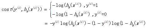
When the actual sample belongs to category 1, if the prediction probability is also 1, the loss is 0 and the prediction is correct. On the contrary, if the prediction is 0, the loss will be infinite. The loss function constructed in this way is reasonable, and it is also a convex function, which is very convenient to obtain the parameters θ， Minimize the loss function J.

3. Optimization

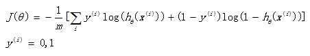
We have defined the loss function J( θ)， The next task is to find the parameters θ. Our goal is very clear, is to find a group θ， So that our loss function J( θ) minimum. There are two commonly used solution methods: batch gradient descent method and Newton's method. Both methods are numerical solutions obtained by iteration, but the convergence speed of Newton iterative method is faster.

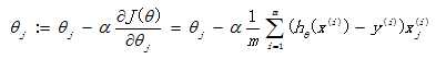
Batch gradient descent method:

Newton iteration method:

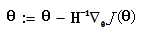
(H is Heather matrix)

4.python code implementation

 1 # -*- coding: utf-8 -*-
 2 """
 3 Created on Wed Feb 24 11:04:11 2016
 4 
 5 @author: SumaiWong
 6 """
 7 
 8 import numpy as np
 9 import pandas as pd
10 from numpy import dot
11 from numpy.linalg import inv
12 
13 iris = pd.read_csv('D:\iris.csv')
14 dummy = pd.get_dummies(iris['Species']) # Generate dummy variables for specifications
15 iris = pd.concat([iris, dummy], axis =1 )
16 iris = iris.iloc[0:100, :] # Intercept the first 100 lines of samples
17 
18 # Construct Logistic Regression and classify whether the disciplines are setosa or not. Setosa ~ sepal Length
19 # Y = g(BX) = 1/(1+exp(-BX))
20 def logit(x):
21     return 1./(1+np.exp(-x))
22 
23 temp = pd.DataFrame(iris.iloc[:, 0])
24 temp['x0'] = 1.
25 X = temp.iloc[:,[1,0]]
26 Y = iris['setosa'].reshape(len(iris), 1) #Sort out the X matrix and Y matrix
27 
28 # Batch gradient descent method
29 m,n = X.shape #Matrix size
30 alpha = 0.0065 #Set learning rate
31 theta_g = np.zeros((n,1)) #Initialization parameters
32 maxCycles = 3000 #Number of iterations
33 J = pd.Series(np.arange(maxCycles, dtype = float)) #loss function 
34 
35 for i in range(maxCycles):
36     h = logit(dot(X, theta_g)) #Estimated value  
37     J[i] = -(1/100.)*np.sum(Y*np.log(h)+(1-Y)*np.log(1-h)) #Calculate loss function value      
38     error = h - Y #error
39     grad = dot(X.T, error) #gradient
40     theta_g -= alpha * grad
41 print theta_g
42 print J.plot()   
43 
44 # Newton’s method 
45 theta_n = np.zeros((n,1)) #Initialization parameters
46 maxCycles = 10 #Number of iterations
47 C = pd.Series(np.arange(maxCycles, dtype = float)) #loss function 
48 for i in range(maxCycles):
49     h = logit(dot(X, theta_n)) #Estimated value 
50     C[i] = -(1/100.)*np.sum(Y*np.log(h)+(1-Y)*np.log(1-h)) #Calculate loss function value      
51     error = h - Y #error
52     grad = dot(X.T, error) #gradient
53     A =  h*(1-h)* np.eye(len(X)) 
54     H = np.mat(X.T)* A * np.mat(X) #Heather matrix, H = X`AX
55     theta_n -= inv(H)*grad
56 print theta_n
57 print C.plot()   

Data download address for code: https://files.cnblogs.com/files/sumai/iris.rar