What is Logistic regression?

         Since the principle of Logistic Regression is to map the results of linear regression (-,) to (0,1) using logical functions, linear regression functions and logical functions are introduced first.                                   

1. Linear Regression Functions

         Mathematical expressions for linear regression functions:

 

         Where xi is an independent variable, y is a dependent variable, and y has a range of (-,u), θ 0 is a constant term, θ i(i=1,2,...,n) is the coefficient to be calculated, with different weights θ I reflects the contribution of independent variables to dependent variables. One-variable first-order equation that we learned in junior middle school: y=a+bx. This regression analysis that only includes one independent variable and one dependent variable is called univariate linear regression analysis. The first-order binary equation in junior middle school: y = a+b1x1+b2x2, the first-order ternary equation: y = a+b1x1+b2x2+b3x3. This regression analysis includes regression analysis of two or more independent variables, called multivariate linear regression analysis. Both univariate and multivariate linear regression analysis are linear regression analysis.

  2.   Logical function (Sigmoid function)

         Sigmoid function mathematical expression:

 

          Image of the Sigmoid function:

         

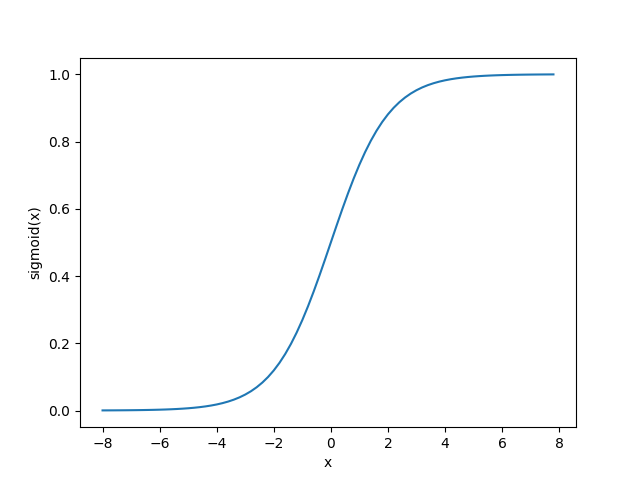
You can see from the image that when x is 0, the Sigmoid function has a value of 0.5. With the increase of x, the corresponding Sigmoid function will approach 1. As x decreases, the value of the Sigmoid function approaches 0, while the Sigmoid function has a range of (0, 1) and the probability P is between 0 and 1, so we can relate the range of Sigmoid to the probability.

3.   Logistic Regression Function  

          The principle of Logistic regression is that the results of linear regression are mapped from (-,u) to (0,1) using the Sigmoid function. Let's describe the above sentence with a formula:

 

By putting the result y of the linear regression function into the sigmod function, a Logistic regression function is constructed.                                 Knowing from the range of Y and the range of sigmod function, the result of linear regression (-,) is mapped to (0,1) by sigmod function in Logistic regression function, which is similar to a probability value.

Let's convert the logistic regression function as follows:

 

Logistic regression is therefore a logarithmic linear model, also known as logarithmic probability regression.

Logistic Regression Classifier

         To implement a logistic regression classifier, we can multiply a regression coefficient on each classification feature and add all the result values together to bring this sum into the sigmoid function. A numerical value in the range 0-1 is obtained. Finally, a threshold value is set, which is 1 when it is greater than the threshold value, or 0 if it is not. That is why logistic regression algorithms are ideas and formulas are functions of classifiers.                                                                                                                                             The logistic classification function is determined. With the classification function, we can input the eigenvectors to get the probability that an instance belongs to a certain category. But there's a problem here, weight(Regression coefficient) We are uncertain. We need to find the best regression coefficient to make the scoring classifier as accurate as possible.                                                                                                                Optimal Regression CoefficientThe maximum likelihood method, Newton method, and optimization method (i.e., the method of gradient rise and gradient decrease) can be used to determine this. The following focuses on the implementation of Logistic regression classification using the gradient-up method.

Gradient Up Algorithm

         The gradient rise method is based on the idea that the best way to find the maximum value of a function is to follow the gradient direction of the function. If the gradient is denoted as_, the gradient of the function f(x,y) is represented by the following:                                                                     

This gradient means moving in the direction of xAnd move in the y directionWhere the function f(x,y) must be defined and probable at the point to be calculated. A specific example of the function is shown in the following figure.

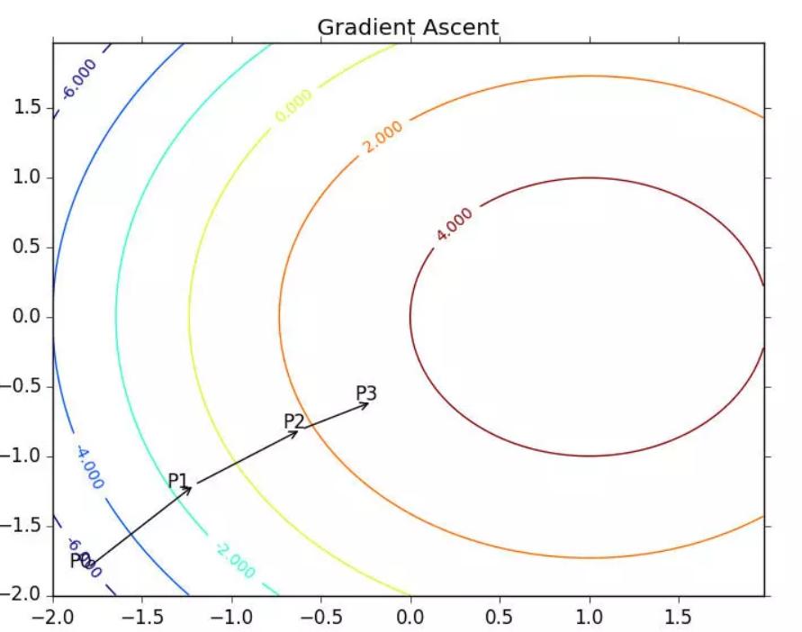
         The gradient-up algorithm reassembles the direction of movement after reaching each point. Beginning with P0, after calculating the gradient of the point, the function moves to the next point P1 according to the gradient. At point P1, the gradient is recalculated again and moved to P2 in the direction of the new gradient. This cycle iterates until the notification condition is met. The gradient operator always ensures that we can choose the best direction of movement during iteration

        The gradient-up algorithm in the figure above moves one step in the direction of the gradient. As you can see, the gradient operator always points in the direction where the function value increases the fastest. What is said here is the direction of movement, not the amount of movement. This value is called the step and is recorded as α \ alpha α. In terms of vectors, the iteration formula of the gradient rise algorithm is as follows:
                                                

           The formula will be iterated until a stop condition is reached, such as the number of iterations reaching a certain value or the algorithm reaching an allowable error range. If the gradient descent method is used, the formula is iterated in the opposite direction of the gradient rise, and the corresponding formula is as follows:                                                                                                                                                                                 

python implementation of gradient rise algorithm

1. General gradient-up algorithm (the entire dataset needs to be traversed each time the regression coefficients (optimal parameters) are updated.)

def gradAscent(dataMatIn, classLabels):#Gradient rise: dataMatIn:2-dimensional NumPy array, 100*3 matrix; classLabels: Class Labels, 1*100 Row Vectors
    dataMatrix = mat(dataMatIn)#Characteristic Matrix
    labelMat = mat(classLabels).transpose()#Class Label Matrix: 100*1 Column Vector
    m,n = shape(dataMatrix)
    alpha = 0.001#Step toward target
    maxCycles = 500#Number of iterations
    weights = ones((n,1))#n*1 column vector: 3 rows 1 column
    for k in range(maxCycles):
        h = sigmoid(dataMatrix*weights)#100*3*3*1=100*1,dataMatrix * weights represents more than one product calculation, actually including 300 products
        error = (labelMat - h)#The difference between the true category and the forecast category
        weights = weights + alpha * dataMatrix.transpose()* error#w:=w+α▽wf(w)
    return weights

  2. Random Gradient Up Algorithm

The general gradient-up algorithm, which traverses the entire dataset every time the regression coefficients are updated, is too complex on billions of samples. Improvement: Random Gradient Up algorithm: Update regression coefficients with only one sample point at a time.)

def stocGradAscent0(dataMatrix, classLabels):
    m, n = shape(dataMatrix)
    alpha = 0.01
    weights = ones(n)
    for i in range(m):
        h = sigmoid(sum(dataMatrix[i] * weights))
        error = classLabels[i] - h
        weights = weights + alpha * error * dataMatrix[i]
    return weights

          Now let's test the classification of these two algorithms with a simple dataset.

The dataset testSet has 100 samples, two attributes x1,x2

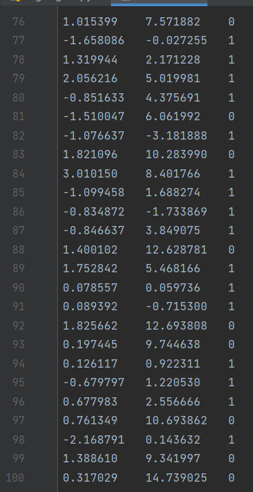
  Complete test code

#coding:utf-8
from numpy import *
import matplotlib.pyplot as plt

class func:
    def loadDataSet(self):
        dataMat = []
        labelMat = []
        fr = open('testSet.txt')
        for line in fr.readlines():
            # Format of Matrix [Label, X1, X2]
            lineArr = line.strip().split()

            #Insert X1, X2, and the initial regression coefficient (weight), all set to 1.0
            dataMat.append([1.0,float(lineArr[0]),float(lineArr[1])])

            #Insert a label,
            #Must be converted to int type because there are only two classes
            labelMat.append(int(lineArr[2]))


        return dataMat,labelMat

    # Classification using sigmoid function
    def sigmoid(self,inX):
        return 1.0/(1+exp(-inX))

    #Normal Gradient Rise
    #Optimize using the gradient rise algorithm to find the optimal optimization factor
    #dataMatIn is a training set, a three-dimensional matrix, (-0.017612) 	 14.053064 	 0)
    #classLabels are class labels, numeric row vectors, which need to be transposed to column vectors with values of 0,1
    def gradAscent(self,dataMatIn,classLabels):
        dataMatrix = mat(dataMatIn) #Convert to Numpy Matrix Data Type
        labelMat = mat(classLabels).transpose() #Transpose matrix for weighted multiplication
        m,n = shape(dataMatrix) #Get the number of rows and columns of the matrix to set the dimension of the weight vector easily

        alpha = 0.001
        maxCycles = 500
        weights = ones((n,1))  #Returns an n * 1 matrix filled with 1 as the initialization weight
        for k in range(maxCycles):
            h = self.sigmoid(dataMatrix*weights)
            erro = (labelMat - h)   #LabelMat is a label derived from the current regression coefficient, labelMat is a label for the training set, and the value is 0,1
            weights = weights + alpha * dataMatrix.transpose( ) * erro  #Change the weight based on the error between the value calculated using the current weight and the initial value.
                                                                        #Adjust regression coefficients in the direction of error
        return weights

    #Random gradient rise

    def stocGradAscent0(dataMatrix, classLabels):
        m, n = shape(dataMatrix)
        alpha = 0.01
        weights = ones(n)
        for i in range(m):
            h = sigmoid(sum(dataMatrix[i] * weights))
            error = classLabels[i] - h
            weights = weights + alpha * error * dataMatrix[i]
         return weights


    def plotBestFit(self,wei):
        weights = wei.getA()
        dataMat,labelMat = self.loadDataSet()
        dataArr = array(dataMat)
        n = shape(dataMat)[0]
        xcord1 = []
        ycord1 = []
        xcord2 = []
        ycord2 = []

        #Draw in two colors depending on the label, easy to distinguish
        for i in range(n):
            if int(labelMat[i]) == 1:
                xcord1.append(dataArr[i,1])
                ycord1.append(dataArr[i,2])
            else :
                xcord2.append(dataArr[i, 1])
                ycord2.append(dataArr[i, 2])

        fig = plt.figure()
        ax = fig.add_subplot(111) #Divide the canvas into rows and columns, and start with the first one
        ax.scatter(xcord1,ycord1,s=30,c='red',marker = 's') #scatter spread
        ax.scatter(xcord2,ycord2,s=30,c='green')
        x = arange(-3.0,3.0,1)
        y = (-weights[0]-weights[1]*x)/weights[2]
        ax.plot(x,y)
        plt.xlabel('x1')
        plt.ylabel('x2')
        plt.show()




if __name__=="__main__":
    #Normal Gradient Rise
    logRegres = func()
    dataArr,labelMat = logRegres.loadDataSet()
    weights = logRegres.gradAscent(dataArr,labelMat)
    logRegres.plotBestFit(weights)


    #Random gradient rise
    logRegres = func()
    dataArr,labelMat = logRegres.loadDataSet()
    weights =stocGradAscent0(array(dataArr),labelMat)
    plotBestFit(weights)

Run Results  

        Normal Gradient Rise

 

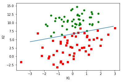
         The classification results are good, and although it is simple and the dataset is small, this method requires a lot of computation (300 multiplies).  

         Random gradient rise  

 

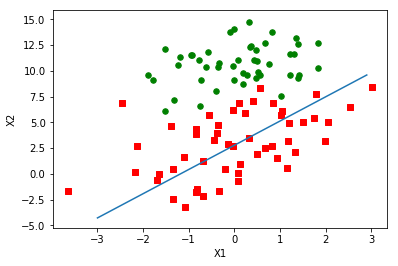
           Fitting results are not as good as the gradient-up algorithm. The classifier here misses one-third of the samples. But the result of the gradient-up algorithm is 500 iterations over the entire dataset. Random gradient rises iterate over the entire dataset 200 times.

         A reliable way to judge whether an optimization algorithm is good or bad: to see if it converges, that is, whether the parameters reach a stable value and are constantly changing. The following figure shows the variation of regression coefficients of the Random Gradient Up algorithm during the 200 iterations. Coefficient 2, or X2, is stable after only 50 iterations, but coefficients 1 and 0 require more iterations.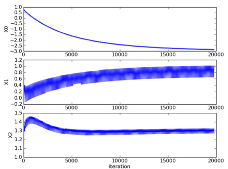

          To solve the problem of under-fitting, we optimize the Random Gradient Up algorithm

# Random Gradient Up Algorithm (Optimized)
def stocGradAscent1(dataMatrix, classLabels, numIter=150):
    m,n = shape(dataMatrix)
    weights = ones(n)   
    
    for j in range(numIter):
        # [0, 1, 2 .. m-1]
        dataIndex = list(range(m))
        for i in range(m):
          
            alpha = 4/(1.0+j+i)+0.0001   
           
            randIndex = int(random.uniform(0,len(dataIndex)))
            # sum(dataMatrix[i]*weights) For the value of f(x), f(x)=a1*x1+b2*x2+. +nn*xn
            h = sigmoid(sum(dataMatrix[randIndex]*weights))
            error = classLabels[randIndex] - h
            # print weights, '__h=%s' % h, '__'*20, alpha, '__'*20, error, '__'*20, dataMatrix[randIndex]
            weights = weights + alpha * error * dataMatrix[randIndex]
            del(dataIndex[randIndex])
    return weights

  Post-run effects

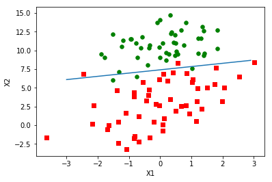
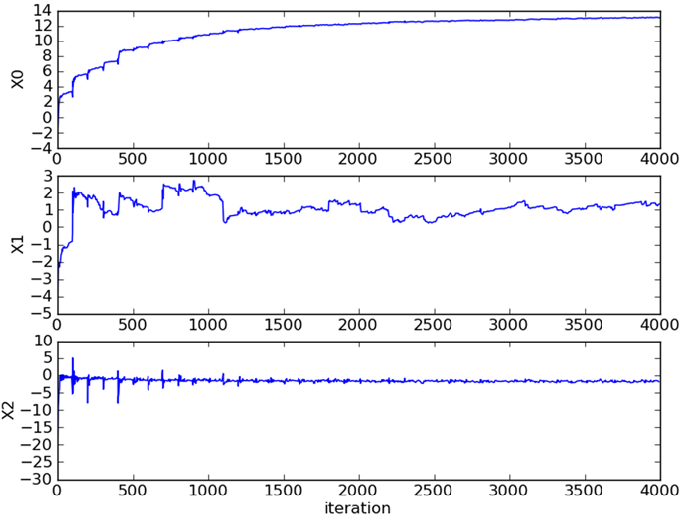
          Random alpha now converges faster than fixed alpha. The main contributions are as follows: 1.stocGradAscent1() avoids periodic fluctuations through its random sampling mechanism; 2.stocGradAscent1() converges faster. This time, the random gradient rise algorithm only traversed the dataset 20 times, whereas the previous normal gradient rise algorithm was 500 times.

          Therefore, when the dataset is small, the gradient-up algorithm can achieve the desired data classification effect. When the dataset is large, in order to effectively reduce the computational load and improve the convergence speed, we use the random gradient rise algorithm.

4 General Processes of Logistic Regression

    (1) Data collection: any method can be used.

    (2) Preparing data: Because distance calculations are required, data types are required to be numeric. Of course, structured data is best formatted.

    (3) Analyzing data: Analyzing data using any method.

    (4) Training algorithm: Most of the time will be used for training, the purpose of training is to find the best regression coefficient for classification.

    (5) Test the algorithm: Once the training phase is completed, the classification will be completed soon.

    (6) Using algorithms: First, some data needs to be input and converted into corresponding structured values; Then, based on the trained regression coefficients, simple regression calculations can be made for these values to determine which category they belong to. Finally, you can do some additional analysis on the categories of output.

Summary of Logistic Regression Models

Advantage:

• The principle is simple, the model is clear, and the operation is efficient. The inference of the probability behind it can withstand speculation. In research, Logistic regression models are often used as a benchmark and more complex algorithms are tried to be used in large data scenarios.
• Update parameters easily using online learning without retraining the entire model.
• Based on probability modeling, the output values fall between 0 and 1 and have probability significance.
• Find out the parameters θ i   Represents the impact of each feature on the output and is highly interpretable.
• The approximate probability predictions of "categories" can be obtained without assuming the distribution of the data in advance (probability values can also be used for subsequent applications). The existing numerical optimization algorithms (such as Newton method) can be used directly to find the optimal solution, which is fast and efficient.

Disadvantages:

• Because of its strong dependence on data, it is necessary to do feature engineering in many cases, and it is mainly used to solve linear separable problems.
• Because it is essentially a linear classifier, it does not handle the correlation between features well and is more sensitive to the multicollinearity of independent variables in the model. For example, two highly correlated independent variables are put into the model at the same time, which may result in a weak independent variable regression symbol not meeting expectations, the symbol being twisted, and the sign changing from positive to negative.
• The logit transformation process is nonlinear and very sensitive with little change rate at both ends and a large change in the middle. Variable changes that result in many intervals have no differentiated effect on the target probability, making it difficult to determine a threshold value.
• Performance is poor when the feature space is large.
• Easy to under-fit, low accuracy.

Scenarios:

• In areas such as P2P, Automotive Finance and so on, based on the information provided by the applicant, predict the likelihood of breach of contract, and then decide whether to lend to the applicant.
• E-commerce platforms predict whether a user will buy a product next time based on the purchase record.
• (Platforms of public opinion such as Tianya, bbs, Weibo, Douban Short Comment are used as emotional classifiers. For example, based on the historical comment data of a netizen on certain topics, it can be predicted whether a netizen will give a positive comment on a certain type of topic next time.
• In the medical field, a patient's tumor is predicted to be benign or malignant based on his or her symptoms.
• Predict whether a suspected patient is truly infected with a new type of coronavirus based on CT, epidemiology, travel history, and test reagent results.
• In the field of precision marketing, forecast the revenue of a product.