Regression algorithm linear regression analysis

Regression: continuous target value

Linear regression: looking for a predictable trend

Linear relationship: two-dimensional, linear relationship; Three dimensional, the target value is in a plane.

linear model

A function predicted by a linear combination of attributes:

linear regression

There is a certain error between the predicted result and the real value

Univariate:

Multivariable:

Loss function (error size)

Try to reduce this loss (two ways) in order to find the W value corresponding to the minimum loss.

Normal equation of least square method

This parameter vector can minimize the cost function.

Gradient descent of least square method

sklearn linear regression normal equation, gradient descent API

Normal equation:

sklearn.linear_model.LinearRegression

Gradient descent:

sklearn.linear_model.SGDRegressor

coef_: regression coefficient

Linear regression example

Boston house price data set analysis process

1. Boston area house price data acquisition

2. Boston area house price data segmentation

3. Standardized processing of training and test data

4. Using the simplest linear regression model, linear regression and
Gradient descent estimation sgdrepressor forecasts house prices

Normal equation:

def mylinear():
    """
    Direct prediction of house price by linear regression
    :return: None
    """
    # get data
    lb = load_boston()

    # Split data set into training set and test set
    x_train, x_test, y_train, y_test = train_test_split(lb.data, lb.target, test_size=0.25)

    print(y_train, y_test)

    # Both eigenvalues and target values must be standardized, and the number of columns is different, so two standardized API s should be instantiated
    std_x = StandardScaler()

    x_train = std_x.fit_transform(x_train)
    x_test = std_x.transform(x_test)

    # target value
    std_y = StandardScaler()

    y_train = std_y.fit_transform(y_train.reshape(-1, 1))
    y_test = std_y.transform(y_test.reshape(-1, 1))

	# estimator prediction
    # Solution of normal equation and prediction results
    lr = LinearRegression()

    lr.fit(x_train, y_train)

    print(lr.coef_)

	# Predict the house price of the test set
    y_lr_predict = std_y.inverse_transform(lr.predict(x_test))

    print("Predicted price of each house in the normal equation test set:", y_lr_predict)

    print("Mean square error of normal equation:", mean_squared_error(std_y.inverse_transform(y_test), y_lr_predict))

	return None

Gradient descent method:

def mylinear():
    """
    Direct prediction of house price by linear regression
    :return: None
    """
    # get data
    lb = load_boston()

    # Split data set into training set and test set
    x_train, x_test, y_train, y_test = train_test_split(lb.data, lb.target, test_size=0.25)

    print(y_train, y_test)

    # Both eigenvalues and target values must be standardized, and the number of columns is different, so two standardized API s should be instantiated
    std_x = StandardScaler()

    x_train = std_x.fit_transform(x_train)
    x_test = std_x.transform(x_test)

    # target value
    std_y = StandardScaler()

    y_train = std_y.fit_transform(y_train.reshape(-1, 1))
    y_test = std_y.transform(y_test.reshape(-1, 1))

	 # Gradient decline to predict house prices
    sgd = SGDRegressor()

    sgd.fit(x_train, y_train)

    print(sgd.coef_)

    # Predict the house price of the test set
    y_sgd_predict = std_y.inverse_transform(sgd.predict(x_test))

    print("Predicted price of each house in gradient descent test set:", y_sgd_predict)

    print("Mean square error of gradient descent:", mean_squared_error(std_y.inverse_transform(y_test), y_sgd_predict))

	renturn None

Regression performance evaluation

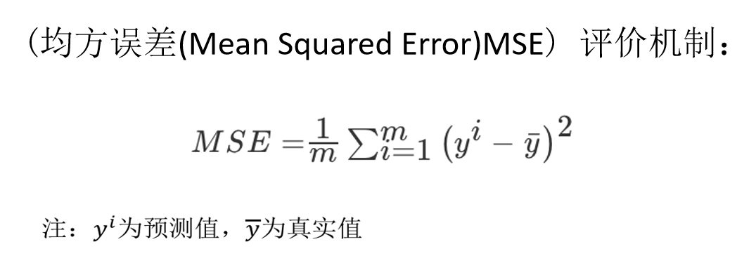
Mean square error API:

sklearn.metrics.mean_squared_error

• mean_squared_error(y_true, y_pred)

Mean square error regression loss

y_true: true value

y_pred: predicted value

return: floating point result

Note: the real value and the predicted value are the values before standardization

LinearRegression and sgdrepressor evaluation

Linear regressor is the most simple and easy-to-use regression model.

However, without knowing the relationship between features, we still use linear regression as the first choice of most systems.

Small scale data: linear regression and others

Large scale data: sgdrepressor

Over fitting and under fitting

The training data is well trained with little error. Why are there problems in the test set

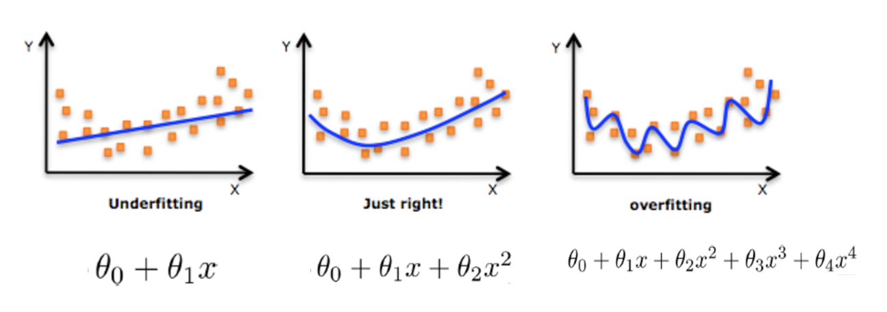
Over fitting: a hypothesis can get better fitting than other hypotheses on the training data, but it can not fit the data well on the data set outside the training data. At this time, it is considered that this hypothesis has over fitting phenomenon. (the model is too complex)

Under fitting: a hypothesis can not get better fitting on the training data, but it can not fit the data well on the data set other than the training data. At this time, it is considered that this hypothesis has the phenomenon of under fitting. (the model is too simple)

Causes and solutions of under fitting

reason:
Too few characteristics of data learned

terms of settlement:
Increase the number of features of the data

Over fitting causes and Solutions

reason:
There are too many original features and some noisy features,
The model is too complex because it tries to take into account
Each test data point

terms of settlement:
Select features to eliminate features with high relevance (difficult to do)
Cross validation (make all data trained)
Regularization (understanding)

L2 regularization

Function: it can make each element of W very small and close to 0

Advantages: the smaller the parameters, the simpler the model is, and the simpler the model is, the less complex it is
Over fitting is easy to occur

Linear regression is prone to over fitting in order to perform the training set data better

L2 regularization: Ridge regression - linear regression with regularization

Linear regression Ridge with regularization

sklearn.linear_model.Ridge

• sklearn.linear_model.Ridge(alpha=1.0)

Linear least squares method with L2 regularization

alpha: regularization strength

coef_: regression coefficient

The greater the regularization, the smaller the weight coefficient

Comparison between linear regression and Ridge

Ridge regression: the regression coefficient obtained by regression is more practical and reliable. In addition, it can make the fluctuation range of estimation parameters smaller and more stable. It has great practical value in the research of too many morbid data.

def mylinear():
    """
    Direct prediction of house price by linear regression
    :return: None
    """
    # get data
    lb = load_boston()

    # Split data set into training set and test set
    x_train, x_test, y_train, y_test = train_test_split(lb.data, lb.target, test_size=0.25)

    print(y_train, y_test)

    # Both eigenvalues and target values must be standardized, and the number of columns is different, so two standardized API s should be instantiated
    std_x = StandardScaler()

    x_train = std_x.fit_transform(x_train)
    x_test = std_x.transform(x_test)

    # target value
    std_y = StandardScaler()

    y_train = std_y.fit_transform(y_train.reshape(-1, 1))
    y_test = std_y.transform(y_test.reshape(-1, 1))

	# Ridge regression to predict house prices
    rd = Ridge(alpha=1.0)

    rd.fit(x_train, y_train)

    print(rd.coef_)

    # Predict the house price of the test set
    y_rd_predict = std_y.inverse_transform(rd.predict(x_test))

    print("Predicted price of each house in ridge regression test set:", y_rd_predict)

    print("Mean square error of ridge regression:", mean_squared_error(std_y.inverse_transform(y_test), y_rd_predict))

    return None