Introduction to linear regression

Linear regression application scenario

House price forecast

Sales quota forecast

Loan line forecast

What is linear regression

Definition and formula

Linear regression is an analytical method that uses regression equation (function) to model the relationship between one or more independent variables (eigenvalues) and dependent variables (target values).

Features: the case with only one independent variable is called univariate regression, and the case with more than one independent variable is called multiple regression



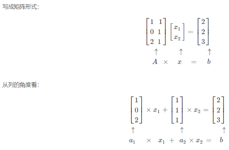
For example:

Final grade: 0.7 × Test score + 0.3 × Usual performance

House price = 0.02 × Distance from central area + 0.04 × Urban nitric oxide concentration + (- 0.12) × Average house price) + 0.254 × Urban crime rate

Analysis of the relationship between the characteristics and objectives of linear regression

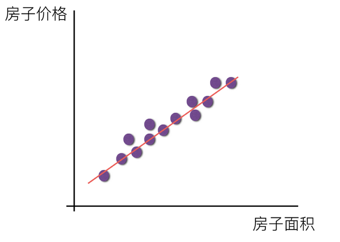
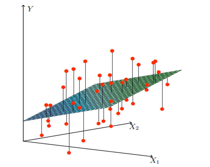
There are two main models in linear regression, one is linear relationship, the other is nonlinear relationship. Here we can only draw a plane for better understanding, so we use a single feature or two features as examples.

Univariate linear relationship:

Multivariable linear relationship:

Nonlinear relationship:

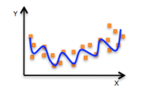
If it is a nonlinear relationship, the regression equation can be understood as:

Derivation

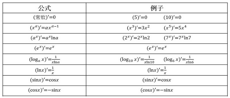
1. Derivatives of common functions

2. Four operations of derivative

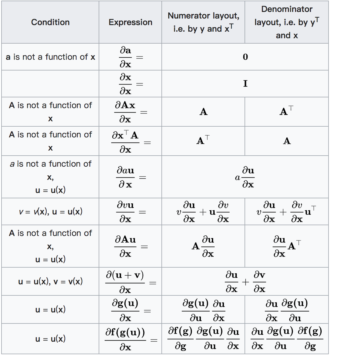
3. Matrix (vector) derivation

Loss and optimization of linear regression

If the real house price has the following relationship:

Real relationship: real house price = 0.02×Distance from central area + 0.04×Urban nitric oxide concentration + (-0.12×Average house price of self owned housing) + 0.254×Urban crime rate

The relationship we randomly specify is:

Random assignment relationship: predicting house prices = 0.25×Distance from central area + 0.14×Urban nitric oxide concentration + 0.42×Average house price of self owned housing + 0.34×Urban crime rate

Then there will be some errors between the predicted value and the real value.
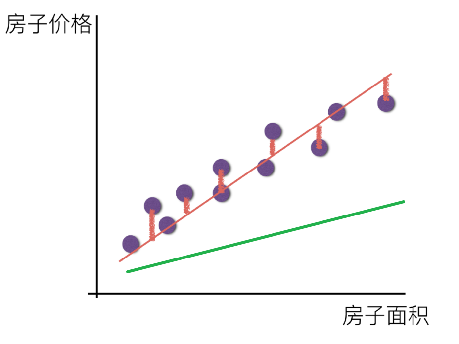Since there is this error, we will measure it.

loss function

Total loss is defined as:

yi is the true value of the ith training sample
h(xi) is the characteristic value combination prediction function of the ith training sample
Also known as least square method

How to reduce this loss and make our prediction more accurate? Since this loss exists, we have always said that machine learning has the function of automatic learning, which can be reflected in linear regression. Here we can use some optimization methods to optimize (actually the derivation function in Mathematics) the total loss of regression!!!

optimization algorithm

How to find w in the model to minimize the loss? (the purpose is to find the W value corresponding to the minimum loss)

Two optimization algorithms are often used in linear regression

Normal equation

Normal equation:

Understanding: X is the eigenvalue matrix and y is the target value matrix. Get the best result directly

Disadvantages: when there are too many and complex features, the solution speed is too slow and the result is not obtained

Derivation of normal equation:

The loss function is converted into matrix writing

Where y is the real value matrix, X is the eigenvalue matrix and w is the weight matrix

For the minimum value of w, the starting and ending y and X are known. The derivative of the quadratic function is obtained directly, and the position where the derivative is zero is the minimum value.

Derivation:

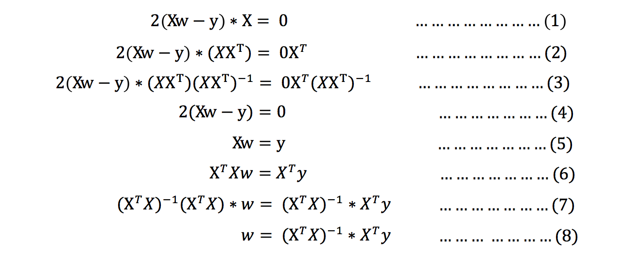
Note: during the derivation of equations (1) to (2), X is a matrix with m rows and n columns, which cannot be guaranteed to have an inverse matrix, but right multiplying XT turns it into a square matrix to ensure that it has an inverse matrix.

In the derivation of equations (5) to (6), it is similar to the above.

Gradient descent

The basic idea of gradient descent method can be compared to a downhill process.

Suppose such a scenario: a person is trapped on a mountain and needs to come down from the mountain (i.e
Find the lowest point of the mountain, that is, the valley). But at this time, the dense fog on the mountain is very large, resulting in low visibility. Therefore, the path down the mountain cannot be determined. He must use the information around him to find the path down the mountain. At this time, he can use the gradient descent algorithm to help himself down the mountain. Specifically, based on his current position, look for the steepest place in this position, and then walk towards the place where the height of the mountain drops, (similarly, if our goal is to climb up the mountain, that is, to climb to the top of the mountain, then we should go up in the steepest direction.) then we will use the same method again and again for each distance, and finally we can successfully reach the valley.

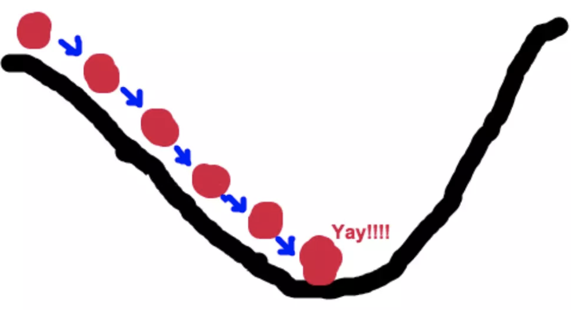
The basic process of gradient descent is very similar to the scene of downhill.

First, we have a differentiable function. This function represents a mountain.

Our goal is to find the minimum value of this function, that is, the bottom of the mountain.

According to the previous scenario assumption, the fastest way to go down the mountain is to find the steepest direction of the current position, and then go down this direction. Corresponding to the function, it is to find the gradient of a given point
Then, in the opposite direction of the gradient, you can make the value of the function drop the fastest! Because the direction of the gradient is the fastest changing direction of the function.
Therefore, we repeatedly use this method to calculate the gradient, and finally we can reach the local minimum, which is similar to the process of going down the mountain. The gradient determines the steepest direction, which is the means to measure the direction in the scene.

Concept of gradient:

Gradient is a very important concept in calculus

In univariate functions, the gradient is actually the differential of the function, representing the slope of the tangent of the function at a given point

In a multivariable function, the gradient is a vector. The vector has a direction. The direction of the gradient points out the fastest rising direction of the function at a given point

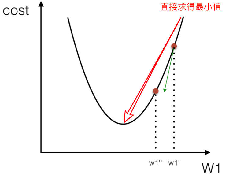
This explains why we need to do everything possible to find the gradient! When we need to reach the bottom of the mountain, we need to observe the steepest place at this time at each step, and the gradient happens to tell us this direction. The direction of the gradient is the fastest rising direction of the function at a given point, and the opposite direction of the gradient is the fastest falling direction of the function at a given point, which is exactly what we need. So as long as we keep walking in the opposite direction of the gradient, we can reach the local lowest point!

Gradient Descent formula:

α What does it mean?

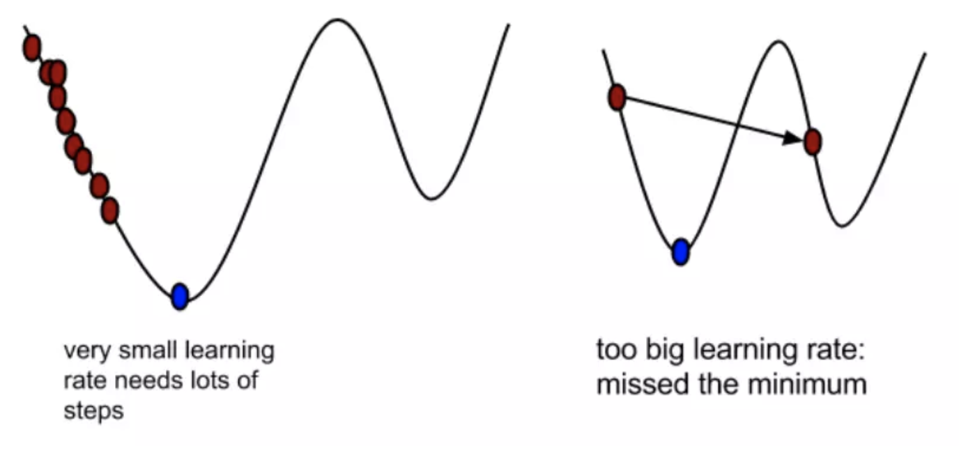
α In gradient descent algorithm, it is called learning rate or step size, which means that we can α To control the distance of each step to ensure that you don't take too big steps. In fact, you don't go too fast and miss the lowest point. At the same time, we should also ensure that we don't walk too slowly, resulting in the sun setting and haven't walked down the mountain yet. therefore α The choice of is often very important in the gradient descent method! α It cannot be too big or too small. If it is too small, it may lead to delay in reaching the lowest point. If it is too big, it will lead to missing the lowest point!

Why is the gradient multiplied by a minus sign?

A minus sign before the gradient means moving in the opposite direction of the gradient! As we mentioned earlier, the direction of the gradient is actually the fastest rising direction of the function at this point! And we need to go in the direction of the fastest descent, which is naturally the direction of the negative gradient, so we need to add a minus sign here

We can better understand the process of gradient descent through two diagrams


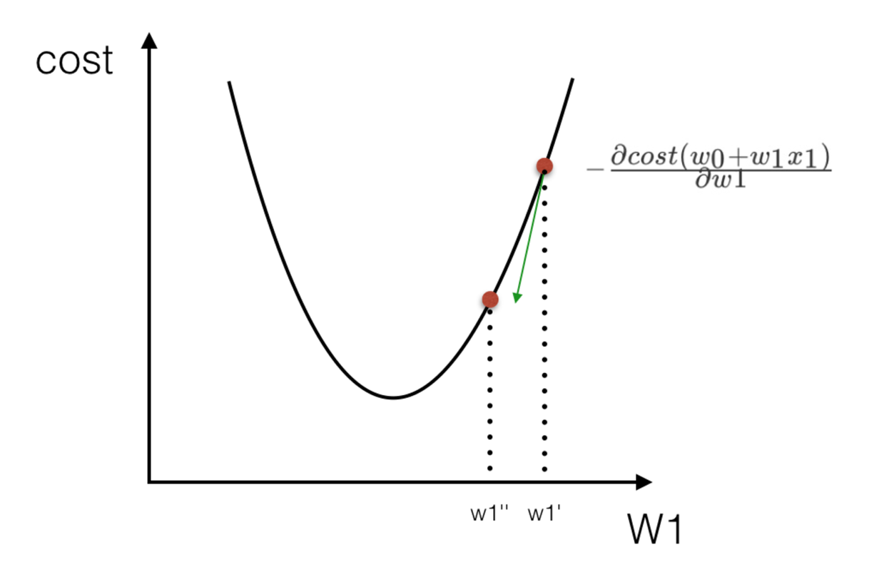
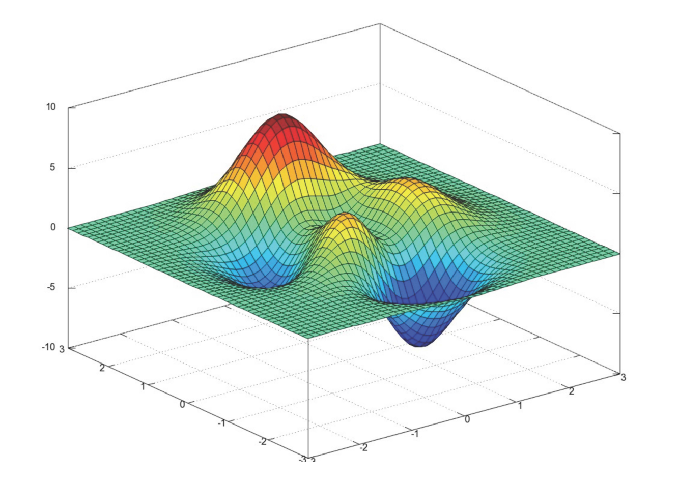
Therefore, with the optimization algorithm of gradient descent, regression has the ability of "automatic learning"

Comparison between gradient descent and normal equation:

gradient descent	Normal equation
Need to select learning rate	unwanted
Iterative solution is required	One operation
A large number of features can be used	Equations need to be calculated, with high time complexity O(n3)

Introduction to gradient descent method

Full gradient descent algorithm (FG)

Calculate all sample errors of the training set, sum them, and then take the average value as the objective function.

The weight vector moves in the opposite direction of its gradient, so as to reduce the current objective function the most.

Because we need to calculate all gradients on the whole dataset during each update, the speed of batch gradient descent method will be very slow. At the same time, batch gradient descent method cannot process datasets that exceed the memory capacity limit.

The batch gradient descent method also can not update the model online, that is, new samples can not be added in the process of operation.

It is to calculate the parameters of the loss function on the whole training data set θ Gradient of:

Random average gradient descent algorithm (SAG)

In the SG method, although the problem of large operation cost is avoided, the SG effect is often unsatisfactory for big data training, because each round of gradient update is completely independent of the data and gradient of the previous round.

The random average gradient algorithm overcomes this problem, maintains an old gradient for each sample in memory, randomly selects the ith sample to update the gradient of this sample, keeps the gradient of other samples unchanged, then obtains the average value of all gradients, and then updates the parameters.

In this way, only one sample gradient needs to be calculated in each round of update, and the calculation cost is equivalent to SG, but the convergence speed is much faster.

Random gradient descent algorithm (SG)

Because FG needs to calculate all sample errors when updating the weight every iteration, and there are often hundreds of millions of training samples in practical problems, it is inefficient and easy to fall into the local optimal solution. Therefore, a random gradient descent algorithm is proposed.

The objective function calculated in each round is no longer the error of all samples, but only the error of a single sample, that is, only the gradient of one sample objective function is calculated to update the weight each time, and then take the next sample and repeat the process until the loss function value stops falling or the loss function value is less than a tolerable threshold.

This process is simple and efficient, and can generally avoid the convergence of update iteration to the local optimal solution. The iterative form is:

Using only one sample iteration at a time, it is easy to fall into local optimal solution in case of noise.

Among them, x(i)Represents the eigenvalue of a training sample, y(i)Represents the tag value of a training sample

However, because SG only uses one sample iteration at a time, it is easy to fall into local optimal solution in case of noise.

Small batch gradient descent algorithm (Mini bantch)

Small batch gradient descent algorithm is a compromise between FG and SG, which takes into account the advantages of the above two methods to a certain extent.

A small sample set is randomly selected from the training sample set each time, and FG iteration is used to update the weight on the extracted small sample set.

The number of sample points contained in the extracted small sample set is called batch_size, usually set to the power of 2, which is more conducive to GPU acceleration. In particular, if batch_ If size = 1, it becomes SG; If batch_size=n, it becomes FG The iterative form is:

Linear regression api

sklearn.linear_model.LinearRegression(fit_intercept=True)

Optimization by normal equation
fit_intercept: calculate offset
LinearRegression.coef_: regression coefficient
LinearRegression.intercept_: bias

sklearn.linear_model.SGDRegressor(loss="squared_loss", fit_intercept=True, learning_rate ='invscaling', eta0=0.01)

Sgdrepressor class implements random gradient descent learning, which supports different loss functions and regularization penalty terms to fit the linear regression model.

Loss: loss type
loss=”squared_ "Loss": ordinary least square method

fit_intercept: calculate offset
learning_rate : string, optional

Learning rate filling
'constant': eta = eta0
'optimal': eta = 1.0 / (alpha * (t + t0)) [default]
'invscaling': eta = eta0 / pow(t, power_t)

power_t=0.25: it exists in the parent class
For the learning rate of a constant value, you can use learning_rate = 'constant', and use eta0 to specify the learning rate.
SGDRegressor.coef_: regression coefficient
SGDRegressor.intercept_: bias

Under fitting and over fitting

definition

Over fitting: one hypothesis can get better fitting than other hypotheses on the training data,
However, it can not fit the data well on the test data set. At this time, it is considered that this hypothesis has been over fitted. (the model is too complex)

Under fitting: a hypothesis can not get a better fit on the training data, and can not fit the data well on the test data set. At this time, it is considered that the hypothesis has a phenomenon of under fitting. (the model is too simple)

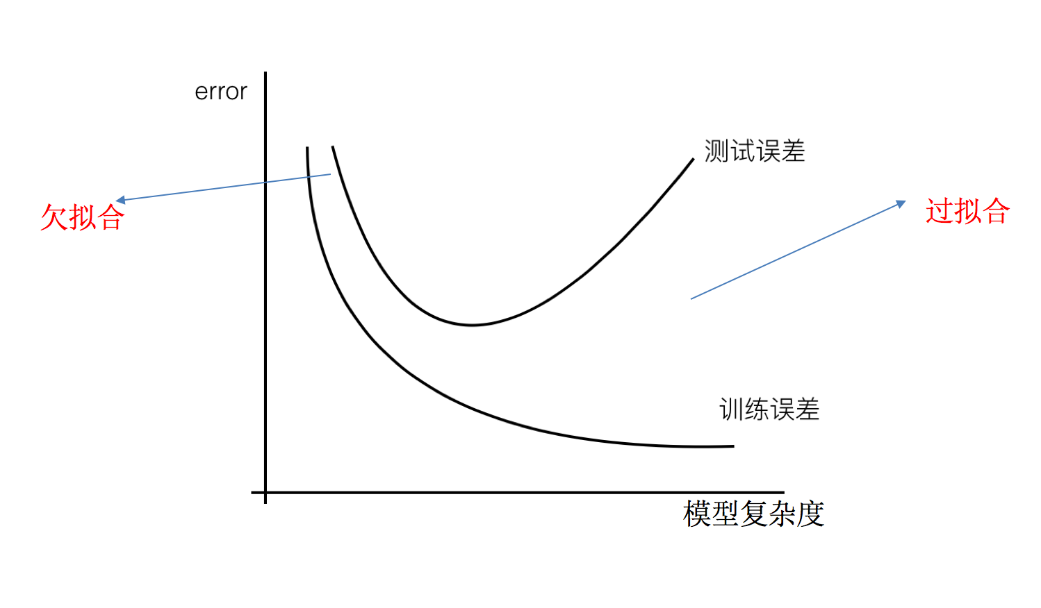
So what makes the model complex? When training and learning linear regression, the model will become complex. Here corresponds to the two relationships of linear regression mentioned above. The data of nonlinear relationship, that is, there are many useless features or the relationship between the characteristics of things in reality and the target value is not a simple linear relationship.

Causes and solutions:

Causes and solutions of under fitting

Reason: too few characteristics of data are learned

terms of settlement:
1. When adding other feature items, sometimes the under fitting of our model is caused by insufficient feature items. You can add other feature items to solve it well. For example, "combination", "generalization" and "relevance" are important means of feature addition. No matter what scene, you can draw gourd and ladle according to gourd, and you will always get unexpected results. In addition to the above features, "context features", "platform features", etc. can be used as preferences for feature addition.
2. Adding polynomial features is very common in machine learning algorithms. For example, adding quadratic or cubic terms to a linear model makes the model more generalized.

Over fitting causes and Solutions

Reason: there are too many original features and some noisy features. The model is too complex because the model tries to take into account all test data points.

terms of settlement:

1. Re cleaning the data may also be caused by impure data. If over fitting occurs, we need to re clean the data.
2. Another reason for increasing the amount of training data is that the amount of data we use for training is too small, and the proportion of training data in the total data is too small.
3. Regularization
4. Reduce feature dimensions and prevent dimension disasters

Regularization

In solving regression over fitting, we choose regularization. However, for other machine learning algorithms such as classification algorithms, such problems will also occur. In addition to the role of some algorithms (decision tree and neural network), we also make feature selection by ourselves, including deleting and merging some features.

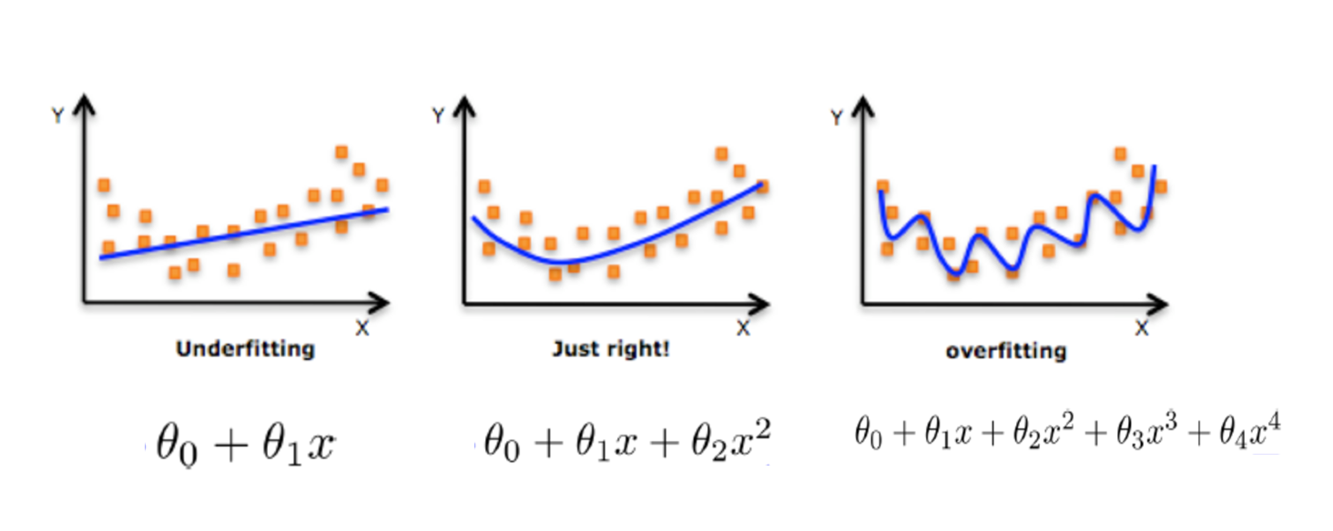
How to solve it?

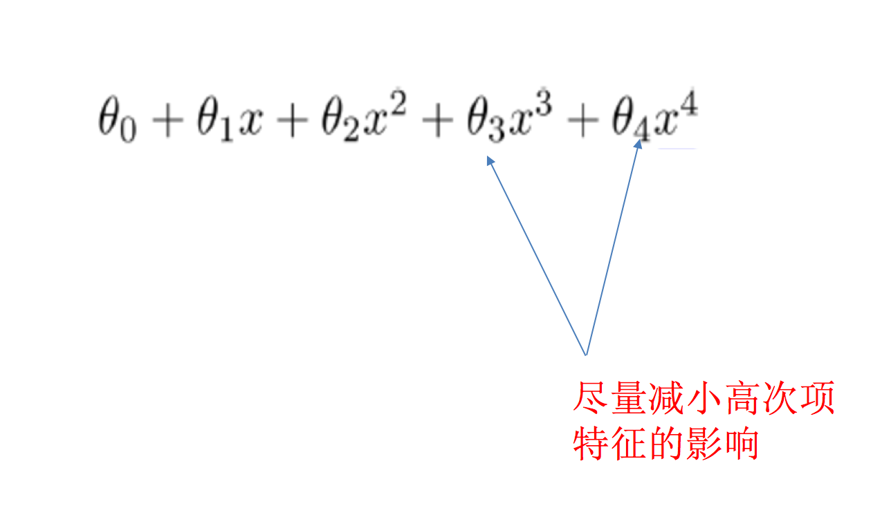
During learning, some features provided by the data affect the model complexity or there are many data points of this feature, so the algorithm tries to reduce the impact of this feature (or even delete the impact of a feature) during learning, which is regularization.

Regularization category:
1. L1 regularization

Function: can make some of them W The value of is directly 0, and the influence of this feature is deleted
LASSO regression

2. L2 regularization

Function: can make some of them W Are very small, close to 0, weakening the impact of a feature
 Advantages: the smaller the parameter, the simpler the model, and the simpler the model, the less likely it is to produce over fitting
Ridge regression

Regularized linear model

Ridge Regression (also known as Tikhonov regularization)

Ridge regression is a regularized version of linear regression, that is, a regularization term is added to the cost function of the original linear regression:
In order to fit the data and make the model weight as small as possible, ridge regression cost function:

α= 0: ridge regression degenerates to linear regression

Lasso regression

Lasso regression is another regularization version of linear regression. The regularization term is ℓ 1 norm of weight vector.

Cost function of Lasso regression:

be careful:

Lasso Regression The cost function of θi=0 Place is not differentiable.
Solution: inθi=0 A sub gradient vector is used at(subgradient vector)Instead of gradient, the following formula
Lasso Regression Subgradient vector of

Lasso Regression has a very important property: it tends to completely eliminate unimportant weights.

For example, when α When the value is relatively large, the higher-order polynomial degenerates to quadratic or even linear: the weight of the characteristics of the higher-order polynomial is set to 0.

In other words, Lasso Regression can automatically select features and output a sparse model (only a few features have non-zero weights).

Elastic Net

The elastic network makes a compromise between ridge regression and Lasso regression, and is controlled by the mix ratio R:
Cost function of elastic network:

r=0: Elastic network becomes ridge regression
r=1: Elastic networks are Lasso regression

Ridge regression api

   sklearn.linear_model.Ridge(alpha=1.0, fit_intercept=True,solver="auto", normalize=False)

    have l2 Regularized linear regression
    alpha:Regularization strength, also known as λ
        λValue: 0~1 1~10
    solver:The optimization method will be automatically selected according to the data
        sag:If the data set and features are large, select the random gradient descent optimization
    normalize:Is the data standardized
        normalize=False:Can be in fit Previous call preprocessing.StandardScaler Standardized data
    Ridge.coef_:Regression weight
    Ridge.intercept_:Regression bias

The Ridge method is equivalent to SGDRegressor(penalty = 'l2', loss = "squared_loss"), but SGDRegressor implements a common random gradient descent learning. It is recommended to use Ridge (SAG)

sklearn.linear_model.RidgeCV(_BaseRidgeCV, RegressorMixin)

Linear regression with l2 regularization can be cross verified
coef_: regression coefficient

Case: Boston house price forecast

Data introduction: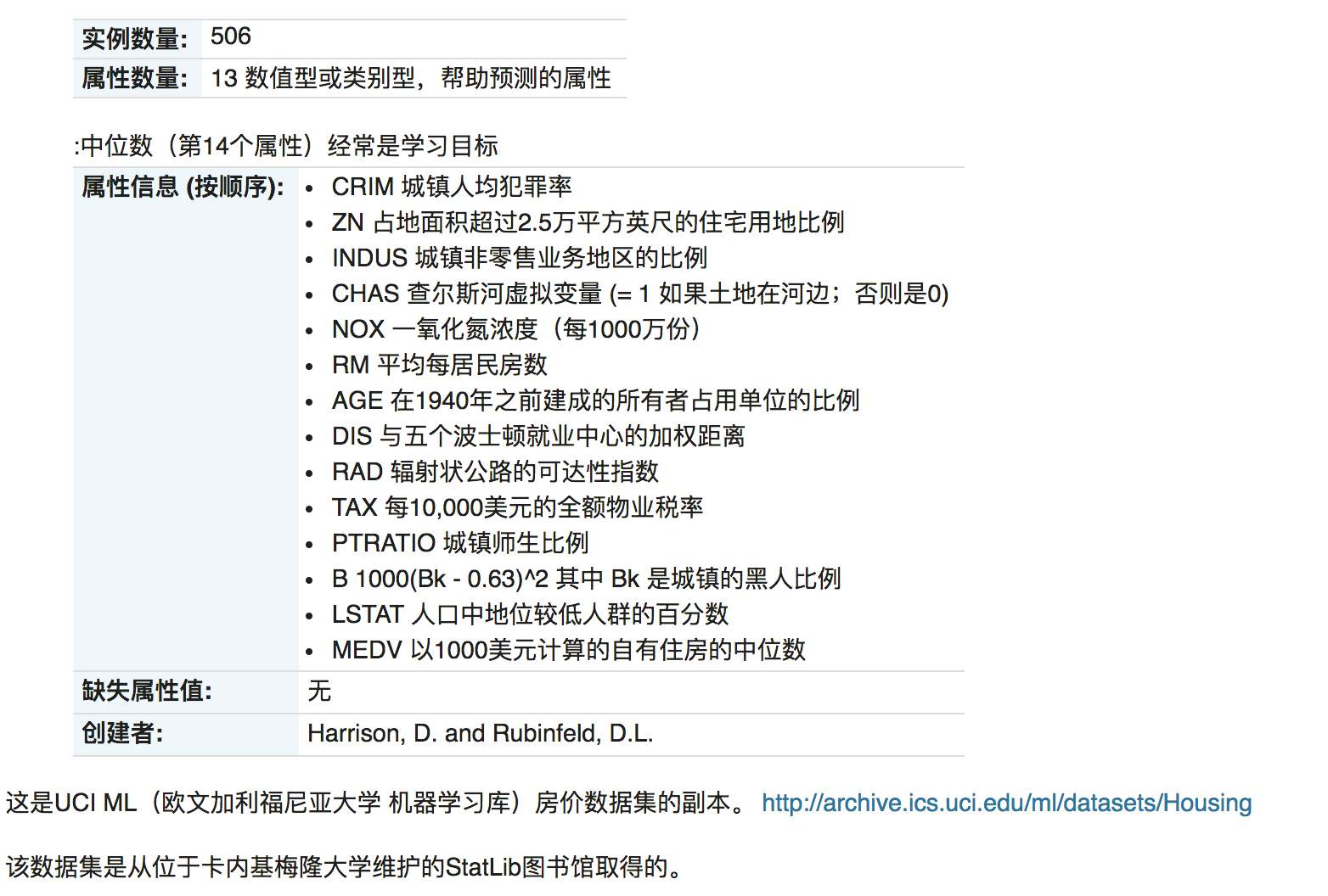

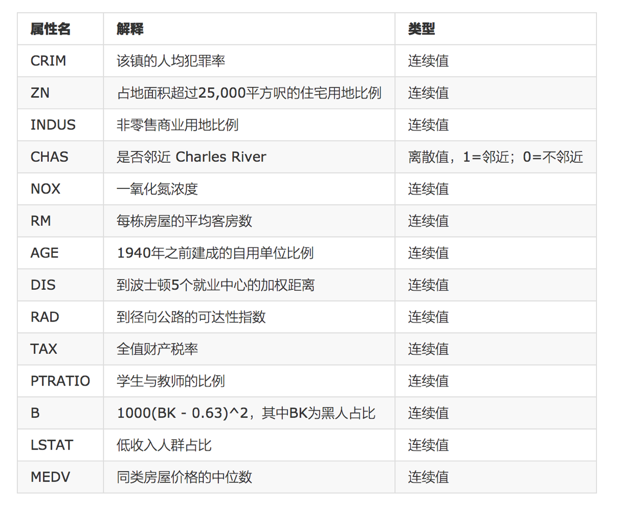
analysis

Whether the inconsistent data size in the regression will have a great impact on the results. Therefore, it needs to be standardized.

Data segmentation and standardization
 Regression prediction
 Effect evaluation of linear regression algorithm

Regression performance evaluation

Mean square error (MSE) evaluation mechanism:

Note: yi is the predicted value and y is the real value

sklearn.metrics.mean_squared_error(y_true, y_pred)
    Mean square error regression loss
    y_true:True value
    y_pred:Estimate
    return:Floating point result

code

from sklearn.datasets import load_boston
from sklearn.model_selection import train_test_split
from sklearn.preprocessing import StandardScaler
from sklearn.linear_model import LinearRegression,SGDRegressor,Ridge,RidgeCV
from sklearn.metrics import mean_squared_error

def linear_model1():
    # Normal equation
    data = load_boston();

    x_train,x_test,y_train,y_test = train_test_split(data.data,data.target,train_size=0.8)

    transfer = StandardScaler()
    x_train = transfer.fit_transform(x_train)
    x_test = transfer.fit_transform(x_test)

    estimator = LinearRegression()
    estimator.fit(x_train,y_train)

    y_predict = estimator.predict(x_test)

    print("The predicted value is:\n",y_predict)
    print("The coefficients in the model are:\n",estimator.coef_)
    print("The offset in the model is:\n",estimator.intercept_)

    print("The accuracy is:\n",estimator.score(x_test,y_test))
    print("Mean square error:\n",mean_squared_error(y_test,y_predict))

    print("Model offset:\n",estimator.intercept_)


def linear_model2():
    # gradient descent 
    data = load_boston();

    x_train,x_test,y_train,y_test = train_test_split(data.data,data.target,train_size=0.8)

    transfer = StandardScaler()
    x_train = transfer.fit_transform(x_train)
    x_test = transfer.fit_transform(x_test)

    estimator = SGDRegressor()
    estimator.fit(x_train,y_train)

    y_predict = estimator.predict(x_test)

    print("The predicted value is:\n",y_predict)
    print("The coefficients in the model are:\n",estimator.coef_)
    print("The offset in the model is:\n",estimator.intercept_)

    print("The accuracy is:\n",estimator.score(x_test,y_test))
    print("Mean square error:\n",mean_squared_error(y_test,y_predict))

    print("Model offset:\n",estimator.intercept_)


def linear_model3():
    # Ridge regression
    data = load_boston();

    x_train,x_test,y_train,y_test = train_test_split(data.data,data.target,train_size=0.8)

    transfer = StandardScaler()
    x_train = transfer.fit_transform(x_train)
    x_test = transfer.fit_transform(x_test)

    estimator = RidgeCV(alphas=(1000,100,10,1,0.1,0.01,0.001))
    estimator.fit(x_train,y_train)

    y_predict = estimator.predict(x_test)

    print("The predicted value is:\n",y_predict)
    print("The coefficients in the model are:\n",estimator.coef_)
    print("The offset in the model is:\n",estimator.intercept_)

    print("The accuracy is:\n",estimator.score(x_test,y_test))
    print("Mean square error:\n",mean_squared_error(y_test,y_predict))

    print("Model offset:\n",estimator.intercept_)

if __name__ == '__main__':
    linear_model1()
    linear_model2()
    linear_model3()

Model saving and loading

Save and load API of sklearn model

from sklearn.externals import joblib

preservation: joblib.dump(estimator, 'test.pkl')
load: estimator = joblib.load('test.pkl')

Note: if importing joblib in skleran fails, you can import joblib directly

import joblib

Linear regression model save load case

from sklearn.datasets import load_boston
from sklearn.model_selection import train_test_split
from sklearn.preprocessing import StandardScaler
from sklearn.linear_model import LinearRegression,SGDRegressor,Ridge,RidgeCV
from sklearn.metrics import mean_squared_error
import joblib

def linear_model3():
    # Ridge regression
    data = load_boston();

    x_train,x_test,y_train,y_test = train_test_split(data.data,data.target,train_size=0.8,random_state=3)

    transfer = StandardScaler()
    x_train = transfer.fit_transform(x_train)
    x_test = transfer.fit_transform(x_test)

    # estimator = RidgeCV(alphas=(1000,100,10,1,0.1,0.01,0.001))
    # estimator.fit(x_train,y_train)
    # joblib.dump(estimator,"test.pkl")
    estimator = joblib.load("test.pkl")

    y_predict = estimator.predict(x_test)

    print("The predicted value is:\n",y_predict)
    print("The coefficients in the model are:\n",estimator.coef_)
    print("The offset in the model is:\n",estimator.intercept_)

    print("The accuracy is:\n",estimator.score(x_test,y_test))
    print("Mean square error:\n",mean_squared_error(y_test,y_predict))

    print("Model offset:\n",estimator.intercept_)

if __name__ == '__main__':
    linear_model3()