Background knowledge required for reading this article: first, lose programming knowledge
1, Introduction
in life, every time we arrive at the meal point, we will silently recite in our hearts, "what are you going to eat later?", Maybe we don't want to go far after working all day today. At this time, we will decide that the distance of the restaurant can't exceed 200 meters, look at the 20 yuan in our wallet, decide to eat no more than 20, and finally order Lanzhou ramen. From the above example, we can see that the Lanzhou Ramen we eat today is determined by a series of previous decisions.
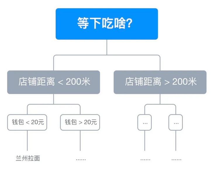
< center > Figure 1-1 < / center >
as shown in Figure 1-1, the above decision process is represented by a binary tree, which is called Decision Tree. In machine learning, the Decision Tree model shown in Figure 1-1 can also be trained through the data set. This algorithm is called Decision Tree Learning algorithm1 .
Two, model introduction
Model
Decision Tree Learning algorithm must first be a tree structure, which is composed of internal nodes and leaf nodes. Internal nodes represent a dimension (feature) and leaf nodes represent a classification. If nodes can be regarded as a pile of decision trees, so they can be connected through a certain set of conditions else... A collection of rules.
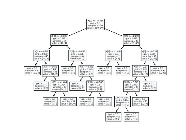
< center > Figure 2-1 < / center >
as shown in Figure 2-1, it shows a basic decision tree data structure and its decision methods.
feature selection
since you want to make a decision, what you need to decide is from which dimension (feature) to make the decision, such as the store distance and the number of change in your wallet in the previous example. In machine learning, we need a quantitative index to determine that the feature used is more appropriate, that is, the "purity" of the subset obtained after using this feature is higher. At this time, three indicators - Information Gain, Gini Index and mean square deviation (MSE) are introduced to solve the above problems.
Information Gain
equation 2-1 is an index representing the purity of the sample set, which is called Information Entropy, where D represents the sample set, K represents the classification number of the sample set, and p_k represents the proportion of the k-th sample in the sample set. The smaller the value of Ent(D), the higher the purity of the sample set.
$$ \operatorname{Ent}(D)=-\sum_{k=1}^{K} p_{k} \log _{2} p_{k} $$
< center > formula 2-1 < / center >
equation 2-2 represents the impact on the sample set after being divided by a discrete attribute, which is called Information Gain, where D represents the sample set, a represents the discrete attribute, v represents the number of all possible values of discrete attribute a, and D^v represents the sub sample set of v value in the sample set.
$$ \operatorname{Gain}(D, a)=\operatorname{Ent}(D)-\sum_{v=1}^{V} \frac{\left|D^{v}\right|}{|D|} \operatorname{Ent}\left(D^{v}\right) $$
< center > formula 2-2 < / center >
when the attribute is a continuous attribute, its available value is not as limited as that of discrete attribute. At this time, the average value of continuous attributes in the sample set can be taken as the division point, and equation 2-2 can be rewritten to obtain the result of equation 2-3, where T_a represents the set of average values, D_t^v represents the subset. When v = -, it represents the subset of samples smaller than the mean value T. when v = +, it represents the subset of samples larger than the mean value T. take the maximum information gain in the partition point as the information gain value of this attribute.
$$ \begin{aligned} T_{a} &=\left\{\frac{a^{i}+a^{i+1}}{2} \mid 1 \leq i \leq n-1\right\} \\ \operatorname{Gain}(D, a) &=\max _{t \in T_{a}} \operatorname{Gain}(D, a, t) \\ &=\max _{t \in T_{a}} \operatorname{Ent}(D)-\sum_{v \in\{-,+\}} \frac{\left|D_{t}^{v}\right|}{|D|} \operatorname{Ent}\left(D_{t}^{v}\right) \end{aligned} $$
< center > formula 2-3 < / center >
The larger the value of Gain(D, a), the higher the purity improvement of the sample set divided according to this attribute. Thus, the most appropriate division attribute can be found, as shown in equation 2-4:
$$ a_{\text {best }}=\underset{a}{\operatorname{argmax}} \operatorname{Gain}(D, a) $$
< center > formula 2-4 < / center >
Gini Index
equation 2-5 is another index representing the purity of the sample set, which is called Gini value, where D represents the sample set, K represents the classification number of the sample set, and p_k represents the proportion of the k-th sample in the sample set. The smaller the value of Gini(D), the higher the purity of the sample set.
$$ \operatorname{Gini}(D)=1-\sum_{k=1}^{K} p_{k}^{2} $$
< center > formula 2-5 < / center >
equation 2-6 represents the impact on the sample set after being divided by a discrete attribute, which is called Gini Index, where D represents the sample set, a represents the discrete attribute, v represents the number of all possible values of discrete attribute a, and D^v represents the sub sample set of v value in the sample set.
$$ \operatorname{Gini_{-}index}(D, a)=\sum_{v=1}^{V} \frac{\left|D^{v}\right|}{|D|} \operatorname{Gini}\left(D^{v}\right) $$
< center > formula 2-6 < / center >
the same as equation 2-3, take the average value of two consecutive attributes as the division point, rewrite equation 2-6, and get the result of equation 2-7, where T_a represents the set of average values, D_t^v represents the subset. When v = -, it represents the subset of samples smaller than the mean value T. when v = +, it represents the subset of samples larger than the mean value T. take the smallest Gini index in the partition point as the Gini index value of this attribute.
$$ \operatorname{Gini_{-}index}(D, a)=\min _{t \in T_{a}} \sum_{v \in\{-,+\}} \frac{\left|D_{t}^{v}\right|}{|D|} \operatorname{Gini}\left(D_{t}^{v}\right) $$
< center > formula 2-7 < / center >
Gini_ The smaller the value of index (D, a), the higher the purity of the sample set divided according to the discrete attribute. Thus, the most appropriate division attribute can be found, as shown in equation 2-8:
$$ a_{\text {best }}=\underset{a}{\operatorname{argmin}} \operatorname{Gini\_index}(D, a) $$
< center > formula 2-8 < / center >
Mean square error (MSE)
the first two indicators enable the decision tree to be used for classification problems. If the decision tree is used for regression problems, different indicators are required to determine the characteristics of division. This indicator is the mean square deviation (MSE) shown in equation 2-9, where T_a represents the set of average values, y_t^v represents the subset label. When v = -, it represents the subset label of the sample smaller than the mean value T. when v = +, it represents the subset label of the sample larger than the mean value T. the latter item is the mean value of the corresponding subset label.
$$ \operatorname{MSE}(D, a)=\min _{t \in T_{a}} \sum_{v \in\{-,+\}}\left(y_{t}^{v}-\hat{y_{t}^{v}}\right)^{2} $$
< center > formula 2-9 < / center >
the smaller the value of MSE(D, a), the higher the fitting degree of the decision tree to the sample set. Thus, the most appropriate division attribute can be found, as shown in equation 2-10:
$$ a_{\text {best }}=\underset{a}{\operatorname{argmin}} \operatorname{MSE}(D, a) $$
< center > formula 2-10 < / center >
knowing the data structure of the decision tree model and how to divide the best data set, let's learn how to generate a decision tree.
3, Algorithm steps
since the data structure of the decision tree is a tree, its child node must also be a tree. The decision tree can be generated recursively. The steps are as follows:
Generate a new node node;
When there is only one category C in the sample:
mark the node node as the leaf node of category C and return the node node;
Traverse all features:
calculate the information gain or Gini index or mean square deviation of the current feature;
Record the best partition feature in node;
After dividing according to the best characteristics, the left part recursively calls the current method as the left child node of the node;
After dividing according to the best characteristics, the right part recursively calls the current method as the right child node of the node;
Return node;
4, Regularization
when the decision tree is generated recursively, the classification of training data by the model will be very accurate, but the performance of unknown prediction data is not ideal. This is the so-called over fitting phenomenon. At this time, the model can be regularized as the solution to over fitting learned by linear regression.
Depth of decision tree
the regularization effect can be achieved by limiting the maximum depth of the decision tree to prevent the decision tree from over fitting. At this time, you only need to add a parameter to record the depth of the current recursive tree in the algorithm step. When the preset maximum depth is reached, no new child nodes will be generated, the current node will be marked as the classification with the largest proportion of classification in the sample, and exit the current recursion.
Leaf node size of decision tree
another method to regularize the decision tree is to limit the minimum number of samples contained in the leaf node, which can also prevent the phenomenon of over fitting. When the number of samples contained in the nodule, mark the current node as the classification with the largest proportion of classification in the sample and exit the current recursion
Pruning of decision tree
the decision tree can also be pruned to prevent over fitting and cut off the redundant subtree. Pruning methods are divided into two types: pre pruning and post pruning.
pre-pruning
as the name suggests, pre pruning is to decide whether to generate sub nodes when generating the decision tree. The judgment method is to use the verification data set to compare the accuracy of generating and not generating sub nodes. When the accuracy of generating sub nodes is improved, the sub nodes are generated, otherwise the sub nodes are not generated.
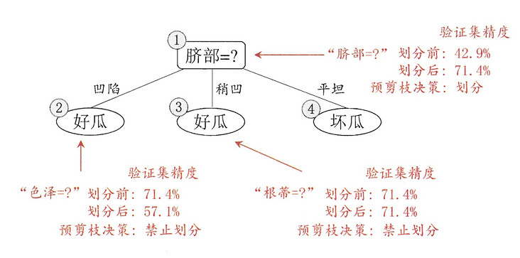
< center > Figure 4-1 is from Zhou Zhihua's machine learning < / center >
post-pruning
post pruning is to form a complete decision tree, and then start from the leaf node. The same judgment method as pre pruning is used. When the accuracy of generating sub nodes is improved, the sub nodes are retained, otherwise the sub nodes are cut off.

< center > Figure 4-2 the picture comes from Zhou Zhihua's machine learning < / center >
5, Code implementation
Implement decision tree classification based on information gain using Python:
import numpy as np

class GainNode:
    """
    Nodes in classification decision tree
    Based on information gain-Information Gain
    """

    def __init__(self, feature=None, threshold=None, gain=None, left=None, right=None):
        # Characteristic subscript of node Division
        self.feature = feature
        # The critical value of node division. When the node is a leaf node, it is the classification value
        self.threshold = threshold
        # Information gain value of node
        self.gain = gain
        # Left node
        self.left = left
        # Right node
        self.right = right

class GainTree:
    """
    Classification decision tree
    Based on information gain-Information Gain
    """

    def __init__(self, max_depth = None, min_samples_leaf = None):
        # Maximum depth of decision tree
        self.max_depth = max_depth
        # Minimum sample number of decision node
        self.min_samples_leaf = min_samples_leaf

    def fit(self, X, y):
        """
        Classification decision tree fitting
        Based on information gain-Information Gain
        """
        y = np.array(y)
        self.root = self.buildNode(X, y, 0)
        return self

    def buildNode(self, X, y, depth):
        """
        Build classification decision tree node
        Based on information gain-Information Gain
        """
        node = GainNode()
        # Return directly when there is no sample
        if len(y) == 0:
            return node
        y_classes = np.unique(y)
        # When there is only one classification in the sample, the classification is returned directly
        if len(y_classes) == 1:
            node.threshold = y_classes[0]
            return node
        # When the depth of the decision tree reaches the maximum depth limit, the classification with the largest proportion of classification in the sample is returned
        if self.max_depth is not None and depth >= self.max_depth:
            node.threshold = max(y_classes, key=y.tolist().count)
            return node
        # When the number of decision leaf node samples reaches the minimum sample limit, the classification with the largest proportion of classification in the sample is returned
        if self.min_samples_leaf is not None and len(y) <= self.min_samples_leaf:
            node.threshold = max(y_classes, key=y.tolist().count)
            return node
        max_gain = -np.inf
        max_middle = None
        max_feature = None
        # Traverse all features to obtain the feature with the largest information gain
        for i in range(X.shape[1]):
            # Calculate the information gain of the feature
            gain, middle = self.calcGain(X[:,i], y, y_classes)
            if max_gain < gain:
                max_gain = gain
                max_middle = middle
                max_feature = i
        # Characteristics of maximum information gain
        node.feature = max_feature
        # critical value
        node.threshold = max_middle
        # information gain
        node.gain = max_gain
        X_lt = X[:,max_feature] < max_middle
        X_gt = X[:,max_feature] > max_middle
        # Recursive processing of left-hand sets
        node.left = self.buildNode(X[X_lt,:], y[X_lt], depth + 1)
        # Recursive processing of right sets
        node.right = self.buildNode(X[X_gt,:], y[X_gt], depth + 1)
        return node

    def calcMiddle(self, x):
        """
        Calculate the average of two continuous features
        """
        middle = []
        if len(x) == 0:
            return np.array(middle)
        start = x[0]
        for i in range(len(x) - 1):
            if x[i] == x[i + 1]:
                continue
            middle.append((start + x[i + 1]) / 2)
            start = x[i + 1]
        return np.array(middle)

    def calcEnt(self, y, y_classes):
        """
        Calculate information entropy
        """
        ent = 0
        for j in range(len(y_classes)):
            p = len(y[y == y_classes[j]])/ len(y)
            if p != 0:
                ent = ent + p * np.log2(p)
        return -ent

    def calcGain(self, x, y, y_classes):
        """
        Calculate information gain
        """
        x_sort = np.sort(x)
        middle = self.calcMiddle(x_sort)
        max_middle = -np.inf
        max_gain = -np.inf
        ent = self.calcEnt(y, y_classes)
        # Traverse each average
        for i in range(len(middle)):
            y_gt = y[x > middle[i]]
            y_lt = y[x < middle[i]]
            ent_gt = self.calcEnt(y_gt, y_classes)
            ent_lt = self.calcEnt(y_lt, y_classes)
            # Calculate information gain
            gain = ent - (ent_gt * len(y_gt) / len(x) + ent_lt * len(y_lt) / len(x))
            if max_gain < gain:
                max_gain = gain
                max_middle = middle[i]
        return max_gain, max_middle

    def predict(self, X):
        """
        Classification decision tree prediction
        """
        y = np.zeros(X.shape[0])
        self.checkNode(X, y, self.root)
        return y

    def checkNode(self, X, y, node, cond = None):
        """
        Judge the classification through the node of classification decision tree
        """
        # When there is no child node, the current critical value is returned directly
        if node.left is None and node.right is None:
            return node.threshold
        X_lt = X[:,node.feature] < node.threshold
        if cond is not None:
            X_lt = X_lt & cond
        # Recursive judgment of left node
        lt = self.checkNode(X, y, node.left, X_lt)
        if lt is not None:
            y[X_lt] = lt
        X_gt = X[:,node.feature] > node.threshold
        if cond is not None:
            X_gt = X_gt & cond
        # Recursive judgment of right node
        gt = self.checkNode(X, y, node.right, X_gt)
        if gt is not None:
            y[X_gt] = gt
Using Python to implement decision tree classification based on Gini index:
import numpy as np

class GiniNode:
    """
    Nodes in classification decision tree
    Based on Gini index-Gini Index
    """

    def __init__(self, feature=None, threshold=None, gini_index=None, left=None, right=None):
        # Characteristic subscript of node Division
        self.feature = feature
        # The critical value of node division. When the node is a leaf node, it is the classification value
        self.threshold = threshold
        # Gini index value of node
        self.gini_index = gini_index
        # Left node
        self.left = left
        # Right node
        self.right = right

class GiniTree:
    """
    Classification decision tree
    Based on Gini index-Gini Index
    """

    def __init__(self, max_depth = None, min_samples_leaf = None):
        # Maximum depth of decision tree
        self.max_depth = max_depth
        # Minimum sample number of decision node
        self.min_samples_leaf = min_samples_leaf

    def fit(self, X, y):
        """
        Classification decision tree fitting
        Based on Gini index-Gini Index
        """
        y = np.array(y)
        self.root = self.buildNode(X, y, 0)
        return self

    def buildNode(self, X, y, depth):
        """
        Build classification decision tree node
        Based on Gini index-Gini Index
        """
        node = GiniNode()
        # Return directly when there is no sample
        if len(y) == 0:
            return node
        y_classes = np.unique(y)
        # When there is only one classification in the sample, the classification is returned directly
        if len(y_classes) == 1:
            node.threshold = y_classes[0]
            return node
        # When the depth of the returned samples reaches the maximum proportion in the classification tree
        if self.max_depth is not None and depth >= self.max_depth:
            node.threshold = max(y_classes, key=y.tolist().count)
            return node
        # When the number of decision leaf node samples reaches the minimum sample limit, the classification with the largest proportion of classification in the sample is returned
        if self.min_samples_leaf is not None and len(y) <= self.min_samples_leaf:
            node.threshold = max(y_classes, key=y.tolist().count)
            return node
        min_gini_index = np.inf
        min_middle = None
        min_feature = None
        # Traverse all features to obtain the feature with the smallest Gini index
        for i in range(X.shape[1]):
            # Gini index for calculating characteristics
            gini_index, middle = self.calcGiniIndex(X[:,i], y, y_classes)
            if min_gini_index > gini_index:
                min_gini_index = gini_index
                min_middle = middle
                min_feature = i
        # Characteristic of minimum Gini index
        node.feature = min_feature
        # critical value
        node.threshold = min_middle
        # gini index
        node.gini_index = min_gini_index
        X_lt = X[:,min_feature] < min_middle
        X_gt = X[:,min_feature] > min_middle
        # Recursive processing of left-hand sets
        node.left = self.buildNode(X[X_lt,:], y[X_lt], depth + 1)
        # Recursive processing of right sets
        node.right = self.buildNode(X[X_gt,:], y[X_gt], depth + 1)
        return node

    def calcMiddle(self, x):
        """
        Calculate the average of two continuous features
        """
        middle = []
        if len(x) == 0:
            return np.array(middle)
        start = x[0]
        for i in range(len(x) - 1):
            if x[i] == x[i + 1]:
                continue
            middle.append((start + x[i + 1]) / 2)
            start = x[i + 1]
        return np.array(middle)

    def calcGiniIndex(self, x, y, y_classes):
        """
        Calculate Gini index
        """
        x_sort = np.sort(x)
        middle = self.calcMiddle(x_sort)
        min_middle = np.inf
        min_gini_index = np.inf
        for i in range(len(middle)):
            y_gt = y[x > middle[i]]
            y_lt = y[x < middle[i]]
            gini_gt = self.calcGini(y_gt, y_classes)
            gini_lt = self.calcGini(y_lt, y_classes)
            gini_index = gini_gt * len(y_gt) / len(x) + gini_lt * len(y_lt) / len(x)
            if min_gini_index > gini_index:
                min_gini_index = gini_index
                min_middle = middle[i]
        return min_gini_index, min_middle

    def calcGini(self, y, y_classes):
        """
        Calculate Gini value
        """
        gini = 1
        for j in range(len(y_classes)):
            p = len(y[y == y_classes[j]])/ len(y)
            gini = gini - p * p
        return gini

    def predict(self, X):
        """
        Classification decision tree prediction
        """
        y = np.zeros(X.shape[0])
        self.checkNode(X, y, self.root)
        return y

    def checkNode(self, X, y, node, cond = None):
        """
        Judge the classification through the node of classification decision tree
        """
        if node.left is None and node.right is None:
            return node.threshold
        X_lt = X[:,node.feature] < node.threshold
        if cond is not None:
            X_lt = X_lt & cond
        lt = self.checkNode(X, y, node.left, X_lt)
        if lt is not None:
            y[X_lt] = lt
        X_gt = X[:,node.feature] > node.threshold
        if cond is not None:
            X_gt = X_gt & cond
        gt = self.checkNode(X, y, node.right, X_gt)
        if gt is not None:
            y[X_gt] = gt
Using Python to realize decision tree regression based on mean square error:
import numpy as np

class RegressorNode:
    """
    Nodes in regression decision tree
    """

    def __init__(self, feature=None, threshold=None, mse=None, left=None, right=None):
        # Characteristic subscript of node Division
        self.feature = feature
        # The critical value of node division. When the node is a leaf node, it is the classification value
        self.threshold = threshold
        # Mean square difference of nodes
        self.mse = mse
        # Left node
        self.left = left
        # Right node
        self.right = right

class RegressorTree:
    """
    Regression decision tree
    """

    def __init__(self, max_depth = None, min_samples_leaf = None):
        # Maximum depth of decision tree
        self.max_depth = max_depth
        # Minimum sample number of decision node
        self.min_samples_leaf = min_samples_leaf

    def fit(self, X, y):
        """
        Regression decision tree fitting
        """
        self.root = self.buildNode(X, y, 0)
        return self

    def buildNode(self, X, y, depth):
        """
        Construct regression decision tree node
        """
        node = RegressorNode()
        # Return directly when there is no sample
        if len(y) == 0:
            return node
        y_classes = np.unique(y)
        # When there is only one classification in the sample, the classification is returned directly
        if len(y_classes) == 1:
            node.threshold = y_classes[0]
            return node
        # When the depth of the decision tree reaches the maximum depth limit, the classification with the largest proportion of classification in the sample is returned
        if self.max_depth is not None and depth >= self.max_depth:
            node.threshold = np.average(y)
            return node
        # When the number of leaves in the decision-making node reaches the minimum classification limit
        if self.min_samples_leaf is not None and len(y) <= self.min_samples_leaf:
            node.threshold = np.average(y)
            return node
        min_mse = np.inf
        min_middle = None
        min_feature = None
        # Traverse all features to obtain the feature with the lowest mean square deviation
        for i in range(X.shape[1]):
            # Calculate the mean square deviation of features
            mse, middle = self.calcMse(X[:,i], y)
            if min_mse > mse:
                min_mse = mse
                min_middle = middle
                min_feature = i
        # Features with minimum mean square deviation
        node.feature = min_feature
        # critical value
        node.threshold = min_middle
        # Mean square deviation
        node.mse = min_mse
        X_lt = X[:,min_feature] < min_middle
        X_gt = X[:,min_feature] > min_middle
        # Recursive processing of left-hand sets
        node.left = self.buildNode(X[X_lt,:], y[X_lt], depth + 1)
        # Recursive processing of right sets
        node.right = self.buildNode(X[X_gt,:], y[X_gt], depth + 1)
        return node

    def calcMiddle(self, x):
        """
        Calculate the average of two continuous features
        """
        middle = []
        if len(x) == 0:
            return np.array(middle)
        start = x[0]
        for i in range(len(x) - 1):
            if x[i] == x[i + 1]:
                continue
            middle.append((start + x[i + 1]) / 2)
            start = x[i + 1]
        return np.array(middle)

    def calcMse(self, x, y):
        """
        Calculate mean square deviation
        """
        x_sort = np.sort(x)
        middle = self.calcMiddle(x_sort)
        min_middle = np.inf
        min_mse = np.inf
        for i in range(len(middle)):
            y_gt = y[x > middle[i]]
            y_lt = y[x < middle[i]]
            avg_gt = np.average(y_gt)
            avg_lt = np.average(y_lt)
            mse = np.sum((y_lt - avg_lt) ** 2) + np.sum((y_gt - avg_gt) ** 2)
            if min_mse > mse:
                min_mse = mse
                min_middle = middle[i]
        return min_mse, min_middle

    def predict(self, X):
        """
        Regression decision tree prediction
        """
        y = np.zeros(X.shape[0])
        self.checkNode(X, y, self.root)
        return y

    def checkNode(self, X, y, node, cond = None):
        """
        Classification is judged by regression decision tree nodes
        """
        if node.left is None and node.right is None:
            return node.threshold
        X_lt = X[:,node.feature] < node.threshold
        if cond is not None:
            X_lt = X_lt & cond
        lt = self.checkNode(X, y, node.left, X_lt)
        if lt is not None:
            y[X_lt] = lt
        X_gt = X[:,node.feature] > node.threshold
        if cond is not None:
            X_gt = X_gt & cond
        gt = self.checkNode(X, y, node.right, X_gt)
        if gt is not None:
            y[X_gt] = gt
6, Third party library implementation
scikit-learn 2 implementation of decision tree classification
from sklearn import tree

# Decision tree classification
clf = tree.DecisionTreeClassifier()
# Fitting data
clf = clf.fit(X, y)
scikit-learn 3 decision tree regression implementation
from sklearn import tree

# Decision tree regression
clf = tree.DecisionTreeRegressor()
# Fitting data
clf = clf.fit(X, y)
7, Animation demonstration
Figure 7-1 shows the classification results of a decision tree without regularization, and figure 7-2 shows the classification results of a regularized decision tree (max_depth = 3, min_samples_leaf = 5)

< center > Figure 7-1 < / center >

< center > figure 7-2 < / center >
figure 7-3 shows the regression results of a decision tree without regularization, and figure 7-4 shows the regression results of a regularized decision tree (max_depth = 3, min_samples_leaf = 5)
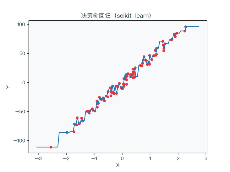
< center > figure 7-3 < / center >
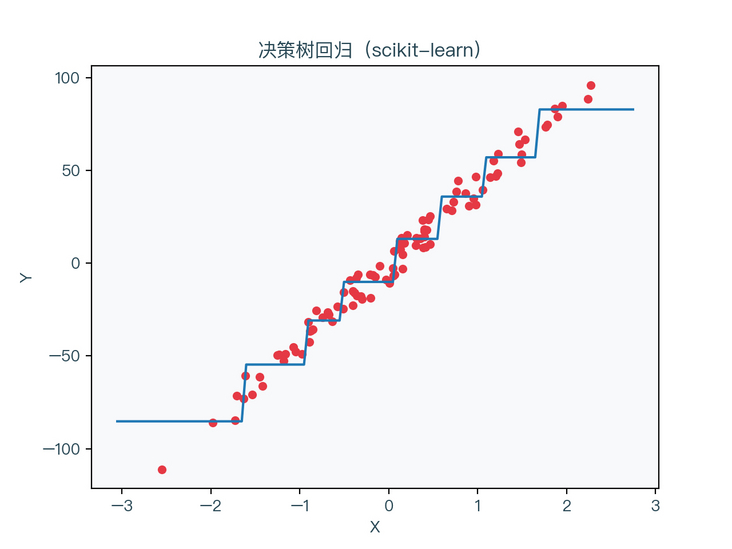
< center > figure 7-4 < / center >
it can be seen that the decision tree without regularization is obviously over fitted to the training data set, and the situation of the regularized decision tree is relatively better.
8, Mind map
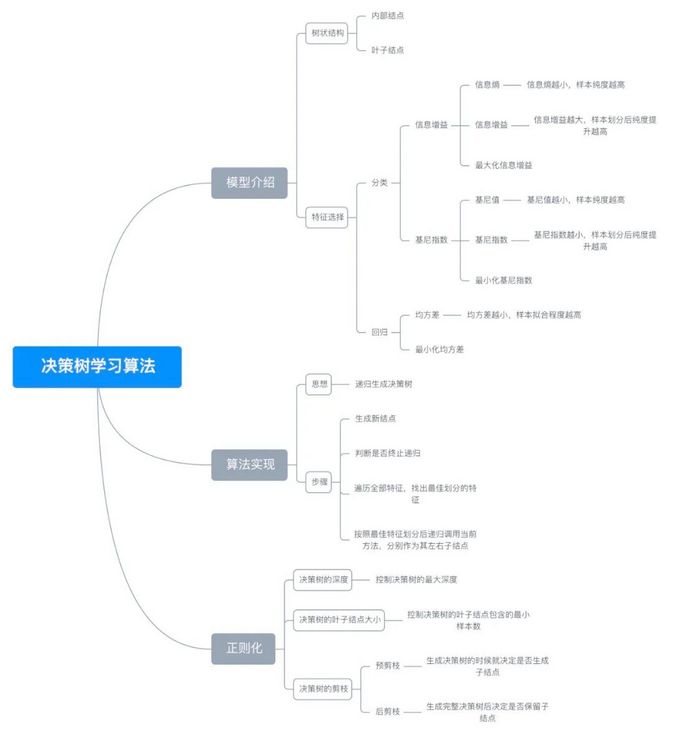
< center > figure 8-1 < / center >
9, References
For a complete demonstration, please click here
Note: This article strives to be accurate and easy to understand, but as the author is also a beginner, his level is limited. If there are errors or omissions in the article, readers are urged to criticize and correct it by leaving a message
This article was first published in—— AI map , welcome to pay attention