Background knowledge required for reading this article: ridge regression, Lasso regression and a little programming knowledge
1, Introduction
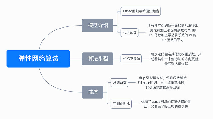
we learned two regularization methods of ridge regression and lasso regression. When multiple features are related, Lasso regression may select only one of them randomly, and ridge regression will select all features. At this time, it is easy to think that if the two regularization methods are combined, the advantages of the two methods can be combined. This regularized algorithm is called Elastic network regression1 (Elastic Net Regression)
Two, model introduction
the cost function of elastic network regression algorithm combines the regularization method of Lasso regression and ridge regression through two parameters λ And ρ To control the size of penalty items.
$$ \operatorname{Cost}(w)=\sum_{i=1}^{N}\left(y_{i}-w^{T} x_{i}\right)^{2}+\lambda \rho\|w\|_{1}+\frac{\lambda(1-\rho)}{2}\|w\|_{2}^{2} $$
also find the size of w when minimizing the cost function:
$$ w=\underset{w}{\operatorname{argmin}}\left(\sum_{i=1}^{N}\left(y_{i}-w^{T} x_{i}\right)^{2}+\lambda \rho\|w\|_{1}+\frac{\lambda(1-\rho)}{2}\|w\|_{2}^{2}\right) $$
you can see that when ρ = When 0, its cost function is equivalent to the cost function of ridge regression ρ = 1, its cost function is equivalent to the cost function of Lasso regression. Like Lasso regression, the absolute value exists in the cost function and is not differentiable everywhere, so there is no way to directly obtain the analytical solution of w by direct derivation, but it can still be used Coordinate descent method 2 (coordinate descent) to solve w.
3, Algorithm steps
Coordinate descent method:
the solution method of coordinate descent method is the same as that of Lasso regression, except that the cost function is different.
specific steps:
(1) Initialize the weight coefficient w, for example, to a zero vector.
(2) Traverse all the weight coefficients, successively take one of the weight coefficients as a variable, fix the other weight coefficients as the result of the previous calculation as a constant, and find the optimal solution under the current condition with only one weight coefficient variable.
in iteration k, the method to update the weight coefficient is as follows:
$$ \begin{matrix} w_m^k represents the k-th iteration and the m-th weight coefficient\ w_1^k = \underset{w_1}{\operatorname{argmin}} \left( \operatorname{Cost}(w_1, w_2^{k-1}, \dots, w_{m-1}^{k-1}, w_m^{k-1}) \right) \\ w_2^k = \underset{w_2}{\operatorname{argmin}} \left( \operatorname{Cost}(w_1^{k}, w_2, \dots, w_{m-1}^{k-1}, w_m^{k-1}) \right) \\ \vdots \\ w_m^k = \underset{w_m}{\operatorname{argmin}} \left( \operatorname{Cost}(w_1^{k}, w_2^{k}, \dots, w_{m-1}^{k}, w_m) \right) \\ \end{matrix} $$
(3) Step (2) is a complete iteration. When all weight coefficients change little or reach the maximum number of iterations, the iteration is ended.
4, Code implementation
Use Python to implement the elastic network regression algorithm (coordinate descent method):
def elasticNet(X, y, lambdas=0.1, rhos=0.5, max_iter=1000, tol=1e-4):
    """
    Elastic network regression, using coordinate descent method( coordinate descent)
    args:
        X - Training data set
        y - Target tag value
        lambdas - Penalty term coefficient
        rhos - Mixed parameter, value range[0,1]
        max_iter - Maximum number of iterations
        tol - Tolerance value of variation
    return:
        w - weight coefficient
    """
    # Initialize w to zero vector
    w = np.zeros(X.shape[1])
    for it in range(max_iter):
        done = True
        # Traverse all arguments
        for i in range(0, len(w)):
            # Record the last round factor
            weight = W[i]
            # Find the best coefficient under the current conditions
            w[i] = down(X, y, w, i, lambdas, rhos)
            # When the variation of one of the coefficients does not reach its tolerance value, continue the cycle
            if (np.abs(weight - w[i]) > tol):
                done = False
        # When all coefficients change little, the cycle ends
        if (done):
            break
    return w

def down(X, y, w, index, lambdas=0.1, rhos=0.5):
    """
    cost(w) = (x1 * w1 + x2 * w2 + ... - y)^2 / 2n + ... + λ * ρ * (|w1| + |w2| + ...) + [λ * (1 - ρ) / 2] * (w1^2 + w2^2 + ...)
    hypothesis w1 Is a variable. At this time, other values are constants. When brought into the above formula, the cost function is about w1 The univariate quadratic function of can be written as follows:
    cost(w1) = (a * w1 + b)^2 / 2n + ... + λρ|w1| + [λ(1 - ρ)/2] * w1^2 + c (a,b,c,λ Are constants)
    => After expansion
    cost(w1) = [aa / 2n + λ(1 - ρ)/2] * w1^2 + (ab / n) * w1 + λρ|w1| + c (aa,ab,c,λ Are constants)
    """
    # Sum of coefficients of quadratic terms after expansion
    aa = 0
    # Sum of coefficients of expanded primary term
    ab = 0
    for i in range(X.shape[0]):
        # Coefficient of the primary term in parentheses
        a = X[i][index]
        # Coefficients of constant terms in parentheses
        b = X[i][:].dot(w) - a * w[index] - y[i]
        # It can be easily obtained that the coefficients of the expanded quadratic term are the sum of the squares of the coefficients of the primary term in parentheses
        aa = aa + a * a
        # It can be easily obtained that the coefficient of the expanded primary term is the coefficient of the primary term in parentheses multiplied by the sum of the constant term in parentheses
        ab = ab + a * b
    # Because it is a univariate quadratic function, when the derivative is zero, the value of the function is the minimum. Only the quadratic term coefficient, the primary term coefficient and λ
    return det(aa, ab, X.shape[0], lambdas, rhos)

def det(aa, ab, n, lambdas=0.1, rhos=0.5):
    """
    Through the derivative of the cost function w,When w = 0 When, non differentiable
    det(w) = [aa / n + λ(1 - ρ)] * w + ab / n + λρ = 0 (w > 0)
    => w = - (ab / n + λρ) / [aa / n  + λ(1 - ρ)]

    det(w) = [aa / n + λ(1 - ρ)] * w + ab / n  - λρ = 0 (w < 0)
    => w = - (ab / n - λρ) / [aa / n  + λ(1 - ρ)]

    det(w) = NaN (w = 0)
    => w = 0
    """
    w = - (ab / n + lambdas * rhos) / (aa / n + lambdas * (1 - rhos))
    if w < 0:
        w = - (ab / n - lambdas * rhos) / (aa / n + lambdas * (1 - rhos))
        if w > 0:
            w = 0
    return w
5, Third party library implementation
scikit-learn 3. Implementation:
from sklearn.linear_model import ElasticNet

# Initialize elastic network regressor
reg = ElasticNet(alpha=0.1, l1_ratio=0.5, fit_intercept=False)
# Fitting linear model
reg.fit(X, y)
# weight coefficient
w = reg.coef_
6, Animation demonstration
the following dynamic diagram shows different ρ Impact on elastic network regression, when ρ When it gradually increases, the L1 regular term dominates, and the closer the cost function is to Lasso regression, when ρ When it decreases gradually, the L2 regular term dominates, and the closer the cost function is to ridge regression.
the following dynamic diagram shows the comparison between Lasso regression and elastic network regression. The dotted line represents the ten features of Lasso regression, the solid line represents the ten features of elastic network regression, and each color represents the weight coefficient of an independent variable (the training data comes from sklearn diabetes datasets)
< center > comparison between lasso regression and elastic network regression < / center >

it can be seen that compared with Lasso regression, elastic network regression retains the nature of feature selection of Lasso regression and takes into account the stability of ridge regression.
7, Mind map
8, References
For a complete demonstration, please click here
Note: This article strives to be accurate and easy to understand, but as the author is also a beginner, his level is limited. If there are errors or omissions in the article, readers are urged to criticize and correct it by leaving a message
This article was first published in—— AI map , welcome to pay attention