Background knowledge required for reading this article: linear regression algorithm and yidui programming knowledge
1, Introduction
in the previous section, we learned that one method to solve multicollinearity is to regularize the cost function. One regularization algorithm is called Ridge Regression Algorithm. Let's learn another regularization algorithm- Lasso regression algorithm )1 (Lasso Regression Algorithm), the full name of LASSO is called least absolute convergence and selection operator.
Two, model introduction
let's first review the cost function of ridge regression, and add a penalty coefficient to the original standard linear regression cost function λ Square of L2 norm of w vector:
$$ \operatorname{Cost}(w) = \sum_{i = 1}^N \left( y_i - w^Tx_i \right)^2 + \lambda\|w\|_{2}^{2} $$
Lasso regression algorithm also adds a regular term like ridge regression, but adds a penalty coefficient instead λ The L1 norm of the w vector is taken as the penalty term (L1 norm means the sum of the absolute values of each element of the vector w), so this regularization method is also called L1 regularization.
$$ \operatorname{Cost}(w) = \sum_{i = 1}^N \left( y_i - w^Tx_i \right)^2 + \lambda\|w\|_1 $$
also find the size of w when minimizing the cost function:
$$ w = \underset{w}{\operatorname{argmin}}\left(\sum_{i = 1}^N \left( y_i - w^Tx_i \right)^2 + \lambda\|w\|_1\right) $$
since the L1 norm of the vector is added, and there is an absolute value, the cost function is not derivable everywhere, so there is no way to directly obtain the analytical solution of w by directly deriving. Here are two methods to solve the weight coefficient w: Coordinate descent method2(coordinate descent),Minimum angle regression3(Least Angle Regression,LARS)
3, Algorithm steps
Coordinate descent method:
the core of coordinate descent method is the same as its name, which is to gradually approach the optimal solution by updating the value of weight coefficient one after another along a certain coordinate axis.
specific steps:
(1) Initialize the weight coefficient w, for example, to a zero vector.
(2) Traverse all the weight coefficients, successively take one of the weight coefficients as a variable, fix the other weight coefficients as the result of the previous calculation as a constant, and find the optimal solution under the current condition with only one weight coefficient variable.
in iteration k, the method to update the weight coefficient is as follows:
$$ \begin{matrix} w_m^k represents the k-th iteration and the m-th weight coefficient\ w_1^k = \underset{w_1}{\operatorname{argmin}} \left( \operatorname{Cost}(w_1, w_2^{k-1}, \dots, w_{m-1}^{k-1}, w_m^{k-1}) \right) \\ w_2^k = \underset{w_2}{\operatorname{argmin}} \left( \operatorname{Cost}(w_1^{k}, w_2, \dots, w_{m-1}^{k-1}, w_m^{k-1}) \right) \\ \vdots \\ w_m^k = \underset{w_m}{\operatorname{argmin}} \left( \operatorname{Cost}(w_1^{k}, w_2^{k}, \dots, w_{m-1}^{k}, w_m) \right) \\ \end{matrix} $$
(3) Step (2) is a complete iteration. When all weight coefficients change little or reach the maximum number of iterations, the iteration is ended.
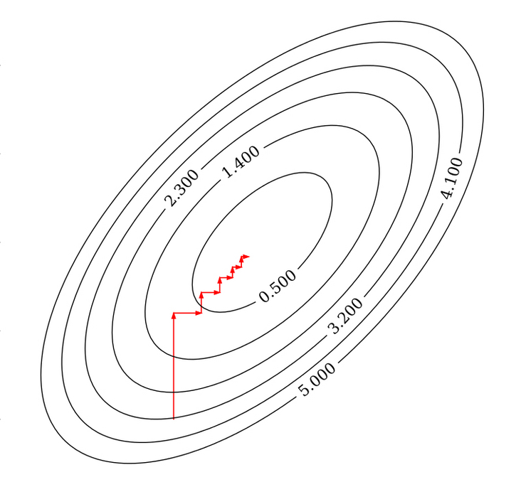
By Nicoguaro - Own work
as shown in the above figure, each iteration fixes other weight coefficients, updates only in the direction of one coordinate axis, and finally reaches the optimal solution.
Minimum angle regression method:
minimum angle regression method is a feature selection method, which calculates the correlation of each feature and gradually calculates the optimal solution through mathematical formula.
specific steps:
(1) Initialize the weight coefficient w, for example, to a zero vector.
(2) Initialize the residual vector as the target label vector y - Xw. Since w is the zero vector at this time, the residual vector is equal to the target label vector y
(3) Select an eigenvector X that has the greatest correlation with the residual vector_ i. Find a set of weight coefficients w along the direction of the eigenvector xi, and another eigenvector x with the largest correlation with the residual vector appears_ J make the correlation between the new residual vector residual and the two eigenvectors equal (that is, the residual vector is equal to the angular bisection vector of the two eigenvectors), and recalculate the residual vector.
(4) Repeat step (3) and continue to find a set of weight coefficients w so that the third eigenvector x with the greatest correlation with the residual vector_ K makes the correlation between the new residual vector residual and the three eigenvectors equal (that is, the residual vector is equal to the equiangular vector of the three eigenvectors), and so on.
(5) When the residual vector residual is small enough or all eigenvectors have been selected, the iteration is ended.
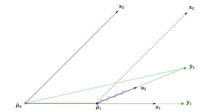
Least Angle Regression - Figure 2
the above figure shows the case when there are only two eigenvectors, and the initial residual vector is y_2, where x_ 1. The correlation between the vector and the residual vector is the largest (the included angle of the vector is the smallest), and find one θ_ 11 so that the new residual vector y_2 - x_ one θ_ 11 is X_ 1 and X_ Angular bisector of 2 (u_2 in the figure), w1 at this time= θ_ 11, w2 = 0. Finally find a group θ_ 21, θ_ 22 so that the new residual vector y_2 - x_ one θ_ 11 - (x_1 θ_ 21 + x_ two θ_ 22) as small as possible, w1= θ_ 11 + θ_ 21,w2 = θ_ 22. All eigenvectors have been selected, so end the iteration.
the coordinate descent method is easier to understand than the minimum angle regression method. You only need to care about one weight coefficient at a time. The minimum angle regression law reduces the number of iterations through some ingenious mathematical formulas, making its worst computational complexity similar to the least square method.
4, Proof of principle
Lasso regression cost function is convex
also need to prove:
$$ f\left(\frac{x_{1}+x_{2}}{2}\right) \leq \frac{f\left(x_{1}\right)+f\left(x_{2}\right)}{2} $$
inequality left:
$$ \operatorname{Cost}\left(\frac{w_{1}+w_{2}}{2}\right)=\sum_{i=1}^{N}\left[\left(\frac{w_{1}+w_{2}}{2}\right)^{T} x_{i}-y_{i}\right]^{2}+\lambda\left\|\frac{w_{1}+w_{2}}{2}\right\|_{1} $$
inequality right:
$$ \frac{\operatorname{Cost}\left(w_{1}\right)+\operatorname{Cost}\left(w_{2}\right)}{2}=\frac{\sum_{i=1}^{N}\left(w_{1}^{T} x_{i}-y_{i}\right)^{2}+\sum_{i=1}^{N}\left(w_{2}^{T} x_{i}-y_{i}\right)^{2}+\lambda\left\|w_{1}\right\|_{1}+\lambda\left\|w_{2}\right\|_{1}}{2} $$
(1) The first half of both sides of the inequality is consistent with the standard linear regression. It only needs to prove that the remaining difference is greater than or equal to zero
(2) According to the positive homogeneity of vector norm, the coefficient of constant term can be multiplied
(3) Will λ Mention outside parentheses
(4) According to the definition of vector norm, if it satisfies the triangular inequality, it must be greater than or equal to zero
$$ \begin{aligned} \Delta &=\lambda\left\|w_{1}\right\|_{1}+\lambda\left\|w_{2}\right\|_{1}-2 \lambda\left\|\frac{w_{1}+w_{2}}{2}\right\|_{1} & (1) \\ &=\lambda\left\|w_{1}\right\|_{1}+\lambda\left\|w_{2}\right\|_{1}-\lambda\left\|w_{1}+w_{2}\right\|_{1} & (2) \\ &=\lambda\left(\left\|w_{1}\right\|_{1}+\left\|w_{2}\right\|_{1}-\left\|w_{1}+w_{2}\right\|_{1}\right) & (3) \\ & \geq 0 & (4) \end{aligned} $$
Artificial control λ The final result must be greater than or equal to zero in the range of real numbers.
Mathematical formula of minimum regression method
find the bisection vector of unit angle:
(1) Let the unit angle bisection vector be u_A. It can be regarded as a linear combination of the selected feature vectors, and the subscript a represents the sequence number set of the selected features
(2) Since the included angle between each selected eigenvector and the angular bisection vector is the same, each element of the vector after the dot product of the eigenvector and the angular bisection vector must be the same, 1_A is a vector whose elements are all 1, and z is a constant
(3) According to equation (2), the coefficient vector of linear combination can be expressed ω_ A
$$ \begin{matrix} u_\mathcal{A} = X_\mathcal{A} \omega_\mathcal{A} & (1)\\ X_\mathcal{A}^Tu_\mathcal{A} = X_\mathcal{A}^TX_\mathcal{A} \omega_\mathcal{A} = z 1_\mathcal{A} & (2)\\ \omega_\mathcal{A} = z(X_\mathcal{A}^TX_\mathcal{A})^{-1} 1_\mathcal{A} & (3) \end{matrix} $$
(1) Angular bisection vector u_A is the unit vector, so the length is 1
(2) Rewrite to vector form
(3) The coefficient vector of the linear combination brought into the previous step ω_ A
(4) According to the property of transpose, the bracket of the first term can be simplified and the constant z is proposed
(5) The matrix multiplied by its inverse matrix is the identity matrix, so it can be simplified
(6) Finally, the expression of constant z is obtained
$$ \begin{array}{cc} \left\|u_{\mathcal{A}}\right\|^{2}=1 & (1)\\ \omega_{\mathcal{A}}^{T} X_{\mathcal{A}}^{T} X_{\mathcal{A}} \omega_{\mathcal{A}}=1 & (2) \\ \left(z\left(X_{\mathcal{A}}^{T} X_{\mathcal{A}}\right)^{-1} 1_{\mathcal{A}}\right)^{T} X_{\mathcal{A}}^{T} X_{\mathcal{A}} z\left(X_{\mathcal{A}}^{T} X_{\mathcal{A}}\right)^{-1} 1_{\mathcal{A}}=1 & (3) \\ z^{2} 1_{\mathcal{A}}^{T}\left(X_{\mathcal{A}}^{T} X_{\mathcal{A}}\right)^{-1}\left(X_{\mathcal{A}}^{T} X_{\mathcal{A}}\right)\left(X_{\mathcal{A}}^{T} X_{\mathcal{A}}\right)^{-1} 1_{\mathcal{A}}=1 & (4) \\ z^21_\mathcal{A}^T\left(X_\mathcal{A}^TX_\mathcal{A}\right)^{-1}1_\mathcal{A} = 1 & (5) \\ z= \frac{1}{\sqrt[]{1_\mathcal{A}^T\left(X_\mathcal{A}^TX_\mathcal{A}\right)^{-1}1_\mathcal{A}}} = \left(1_\mathcal{A}^T\left(X_\mathcal{A}^TX_\mathcal{A}\right)^{-1}1_\mathcal{A}\right)^{-\frac{1}{2} } & (6) \\ \end{array} $$
(1) Multiply the transpose of the eigenvector by the eigenvector and use G_A means
(2) Bring in G_A. Get the expression of z
(3) Bring in G_A. Get ω_ Expression for a
$$ \begin{array}{c} G_{\mathcal{A}}=X_{\mathcal{A}}^{T} X_{\mathcal{A}} & (1)\\ z=\left(1_{\mathcal{A}}^{T}\left(G_{\mathcal{A}}\right)^{-1} 1_{\mathcal{A}}\right)^{-\frac{1}{2}} & (2)\\ \omega_{\mathcal{A}}=z\left(G_{\mathcal{A}}\right)^{-1} 1_{\mathcal{A}} & (3) \end{array} $$
put X_A times ω_ A. You get the angular bisection vector u_A, so that the unit angle bisection vector can be obtained. For more detailed proof, please refer to Bradley Efron's paper4.
find the length of the angular bisector vector:
(1) μ_ A represents the current predicted value and updates one along the direction of the angular bisection vector γ length
(2) C represents the correlation between the eigenvector and the residual vector, which is the dot product of the two vectors. Bring it into equation (1) to obtain the updated expression of the correlation
(3) When the eigenvector is the selected eigenvector, because the product of each eigenvector and angular bisection vector is the same, it is equal to z
(4) Calculate the product of each eigenvector and the angular bisection vector
(5) When the feature vector is not the selected feature vector, use a to bring in equation (2)
(6) If you want to add the next eigenvector, the absolute values of equations (3) and (5) must be equal to ensure that the correlation after the next update is also the same
(7) Solution γ Expression for
$$ \begin{array}{c} \mu_{A^{+}}=\mu_{A}+\gamma u_{A} & (1)\\ C_{+}=X^{T}\left(y-\mu_{A^{+}}\right)=X^{T}\left(y-\mu_{A}-\gamma u_{A}\right)=C-\gamma X^{T} u_{A} & (2)\\ C_{+}=C-\gamma z \quad(j \in A) & (3)\\ a=X^{T} u_{A} & (4)\\ C_{+}=C_{j}-\gamma a_{j} \quad(j \notin A) & (5)\\ |C-\gamma z|=\left|C-\gamma a_{j}\right| & (6)\\ \gamma=\min _{j \notin A}^{+}\left\{\frac{C-C_{j}}{z-a_{j}}, \frac{C+C_{j}}{z+a_{j}}\right\} & (7) \end{array} $$
8195 γ That is, the length of the angular bisector vector. For more detailed proof, please refer to Bradley Efron's paper4.
5, Code implementation
Lasso regression algorithm (coordinate descent method) is implemented in Python:
def lassoUseCd(X, y, lambdas=0.1, max_iter=1000, tol=1e-4):
    """
    Lasso Regression, using coordinate descent method( coordinate descent)
    args:
        X - Training data set
        y - Target tag value
        lambdas - Penalty term coefficient
        max_iter - Maximum number of iterations
        tol - Tolerance value of variation
    return:
        w - weight coefficient
    """
    # Initialize w to zero vector
    w = np.zeros(X.shape[1])
    for it in range(max_iter):
        done = True
        # Traverse all arguments
        for i in range(0, len(w)):
            # Record the last round factor
            weight = w[i]
            # Find the best coefficient under the current conditions
            w[i] = down(X, y, w, i, lambdas)
            # When the variation of one of the coefficients does not reach its tolerance value, continue the cycle
            if (np.abs(weight - w[i]) > tol):
                done = False
        # When all coefficients change little, the cycle ends
        if (done):
            break
    return w

def down(X, y, w, index, lambdas=0.1):
    """
    cost(w) = (x1 * w1 + x2 * w2 + ... - y)^2 + ... + λ(|w1| + |w2| + ...)
    hypothesis w1 Is a variable. At this time, other values are constants. When brought into the above formula, the cost function is about w1 The univariate quadratic function of can be written as follows:
    cost(w1) = (a * w1 + b)^2 + ... + λ|w1| + c (a,b,c,λ Are constants)
    => After expansion
    cost(w1) = aa * w1^2 + 2ab * w1 + λ|w1| + c (aa,ab,c,λ Are constants)
    """
    # Sum of coefficients of quadratic terms after expansion
    aa = 0
    # Sum of coefficients of expanded primary term
    ab = 0
    for i in range(X.shape[0]):
        # Coefficient of the primary term in parentheses
        a = X[i][index]
        # Coefficients of constant terms in parentheses
        b = X[i][:].dot(w) - a * w[index] - y[i]
        # It can be easily obtained that the coefficients of the expanded quadratic term are the sum of the squares of the coefficients of the primary term in parentheses
        aa = aa + a * a
        # It can be easily obtained that the coefficient of the expanded primary term is the coefficient of the primary term in parentheses multiplied by the sum of the constant term in parentheses
        ab = ab + a * b
    # Because it is a univariate quadratic function, when the derivative is zero, the value of the function is the minimum. Only the quadratic term coefficient, the primary term coefficient and λ
    return det(aa, ab, lambdas)

def det(aa, ab, lambdas=0.1):
    """
    Through the derivative of the cost function w,When w = 0 When, non differentiable
    det(w) = 2aa * w + 2ab + λ = 0 (w > 0)
    => w = - (2 * ab + λ) / (2 * aa)

    det(w) = 2aa * w + 2ab - λ = 0 (w < 0)
    => w = - (2 * ab - λ) / (2 * aa)

    det(w) = NaN (w = 0)
    => w = 0
    """
    w = - (2 * ab + lambdas) / (2 * aa)
    if w < 0:
        w = - (2 * ab - lambdas) / (2 * aa)
        if w > 0:
            w = 0
    return w
Lasso regression algorithm (minimum angle regression method) is implemented in Python:
def lassoUseLars(X, y, lambdas=0.1, max_iter=1000):
    """
    Lasso Regression, using the minimum angle regression method( Least Angle Regression)
    Thesis: https://web.stanford.edu/~hastie/Papers/LARS/LeastAngle_2002.pdf
    args:
        X - Training data set
        y - Target tag value
        lambdas - Penalty term coefficient
        max_iter - Maximum number of iterations
    return:
        w - weight coefficient
    """
    n, m = X.shape
    # Selected feature subscript
    active_set = set()
    # Current prediction vector
    cur_pred = np.zeros((n,), dtype=np.float32)
    # residual vector
    residual = y - cur_pred
    # The point product of eigenvector and residual vector, i.e. correlation
    cur_corr = X.T.dot(residual)
    # Select the most relevant subscript
    j = np.argmax(np.abs(cur_corr), 0)
    # Adds a subscript to the selected feature subscript set
    active_set.add(j)
    # Initialize weight coefficient
    w = np.zeros((m,), dtype=np.float32)
    # Record the last weight factor
    prev_w = np.zeros((m,), dtype=np.float32)
    # Record feature update direction
    sign = np.zeros((m,), dtype=np.int32)
    sign[j] = 1
    # Average correlation
    lambda_hat = None
    # Record the last average correlation
    prev_lambda_hat = None
    for it in range(max_iter):
        # Calculate residual vector
        residual = y - cur_pred
        # Point product of eigenvector and residual vector
        cur_corr = X.T.dot(residual)
        # Current correlation maximum
        largest_abs_correlation = np.abs(cur_corr).max()
        # Calculate current average correlation
        lambda_hat = largest_abs_correlation / n
        # When the average correlation is less than λ End the iteration ahead of time
        # https://github.com/scikit-learn/scikit-learn/blob/2beed55847ee70d363bdbfe14ee4401438fba057/sklearn/linear_model/_least_angle.py#L542
        if lambda_hat <= lambdas:
            if (it > 0 and lambda_hat != lambdas):
                ss = ((prev_lambda_hat - lambdas) / (prev_lambda_hat - lambda_hat))
                # Recalculate weight factor
                w[:] = prev_w + ss * (w - prev_w)
            break
        # Update last average correlation
        prev_lambda_hat = lambda_hat

        # When all features are selected, the iteration ends
        if len(active_set) > m:
            break

        # Selected eigenvector
        X_a = X[:, list(active_set)]
        # X in the paper_ Calculation formula of a - (2.4)
        X_a *= sign[list(active_set)]
        # G in the paper_ Calculation formula of a - (2.5)
        G_a = X_a.T.dot(X_a)
        G_a_inv = np.linalg.inv(G_a)
        G_a_inv_red_cols = np.sum(G_a_inv, 1)
        # A in the paper_ Calculation formula of a - (2.5)
        A_a = 1 / np.sqrt(np.sum(G_a_inv_red_cols))
        # In the paper ω  Calculation formula for - (2.6)
        omega = A_a * G_a_inv_red_cols
        # Calculation formula of angular bisection vector in the paper - (2.6)
        equiangular = X_a.dot(omega)
        # Calculation formula of a in the paper - (2.11)
        cos_angle = X.T.dot(equiangular)
        # In the paper γ
        gamma = None
        # Next selected feature subscript
        next_j = None
        # Direction of next feature
        next_sign = 0
        for j in range(m):
            if j in active_set:
                continue
            # In the paper γ  Calculation method of - (2.13)
            v0 = (largest_abs_correlation - cur_corr[j]) / (A_a - cos_angle[j]).item()
            v1 = (largest_abs_correlation + cur_corr[j]) / (A_a + cos_angle[j]).item()
            if v0 > 0 and (gamma is None or v0 < gamma):
                gamma = v0
                next_j = j
                next_sign = 1
            if v1 > 0 and (gamma is None or v1 < gamma):
                gamma = v1
                next_j = j
                next_sign = -1
        if gamma is None:
            # In the paper γ  Calculation method of - (2.21)
            gamma = largest_abs_correlation / A_a

        # Selected eigenvector
        sa = X_a
        # Angular bisection vector
        sb = equiangular * gamma
        # Solving linear equations (sa * sx = sb)
        sx = np.linalg.lstsq(sa, sb)
        # Record the last weight factor
        prev_w = w.copy()
        d_hat = np.zeros((m,), dtype=np.int32)
        for i, j in enumerate(active_set):
            # Update the current weight factor
            w[j] += sx[0][i] * sign[j]
            # D in the paper_ Calculation method of hat - (3.3)
            d_hat[j] = omega[i] * sign[j]
        # In the paper γ_ Calculation method of j - (3.4)
        gamma_hat = -w / d_hat
        # In the paper γ_ Calculation method of hat - (3.5)
        gamma_hat_min = float("+inf")
        # In the paper γ_ Subscript of hat
        gamma_hat_min_idx = None
        for i, j in enumerate(gamma_hat):
            if j <= 0:
                continue
            if gamma_hat_min > j:
                gamma_hat_min = j
                gamma_hat_min_idx = i
        if gamma_hat_min < gamma:
            # Update current forecast vector - (3.6)
            cur_pred = cur_pred + gamma_hat_min * equiangular
            # Remove the subscript to the selected feature subscript set
            active_set.remove(gamma_hat_min_idx)
            # Update feature update direction set
            sign[gamma_hat_min_idx] = 0
        else:
            # Update current prediction vector
            cur_pred = X.dot(w)
            # Adds a subscript to the selected feature subscript set
            active_set.add(next_j)
            # Update feature update direction set
            sign[next_j] = next_sign

    return w
6, Third party library implementation
scikit-learn 6 realization (coordinate descent method):
from sklearn.linear_model import Lasso

# Initialize Lasso regressor. Coordinate descent method is used by default
reg = Lasso(alpha=0.1, fit_intercept=False)
# Fitting linear model
reg.fit(X, y)
# weight coefficient
w = reg.coef_
scikit-learn 7 implementation (minimum angle regression method):
from sklearn.linear_model import LassoLars

# Initialize Lasso regressor and use the minimum angle regression method
reg = LassoLars(alpha=0.1, fit_intercept=False)
# Fitting linear model
reg.fit(X, y)
# weight coefficient
w = reg.coef_
7, Animation demonstration
the following dynamic diagram shows the example of working years and average monthly salary in the previous section. Each time, the weight coefficient is changed only in one direction of this coordinate axis to gradually approach the optimal solution.
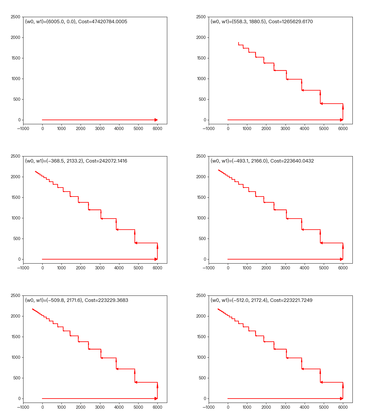
< center > coordinate descent method < / center >
the following dynamic diagram shows λ The horizontal axis is the penalty coefficient λ , The vertical axis is the weight coefficient, and each color represents the weight coefficient of an independent variable (the training data comes from sklearn diabetes datasets):
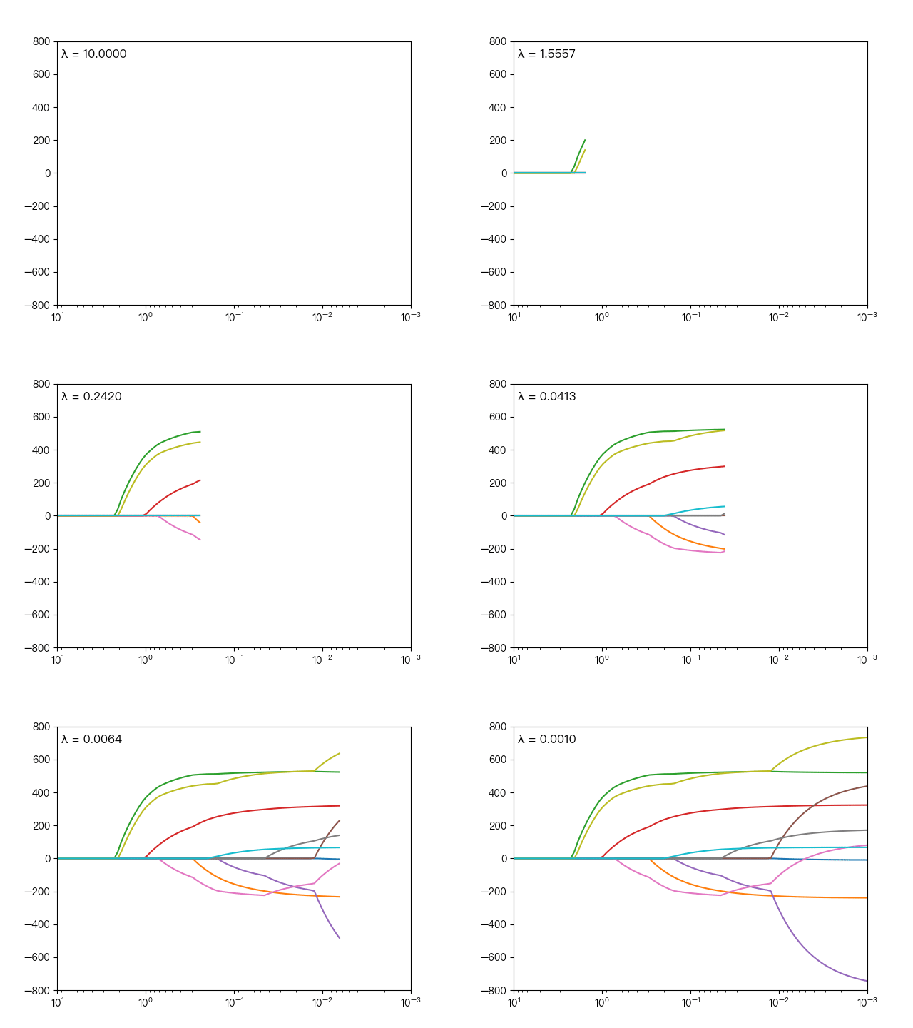
<center> λ Influence on weight coefficient < / center >
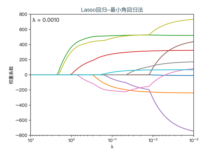
you can see when λ When gradually increasing( λ Moving to the left), the weight coefficient of some features will quickly become zero. This property shows that Lasso regression can be used for feature selection and control λ To select the key features.
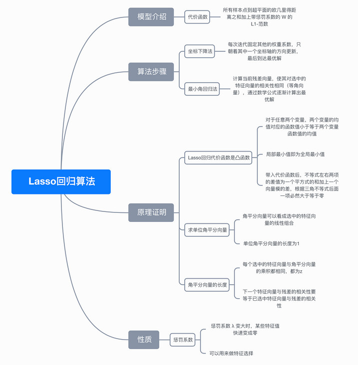
8, Mind map
9, References
- https://en.wikipedia.org/wiki...(statistics)
- https://en.wikipedia.org/wiki...
- https://en.wikipedia.org/wiki...
- https://web.stanford.edu/~has...
- https://zhuanlan.zhihu.com/p/...
- https://scikit-learn.org/stab...
- https://scikit-learn.org/stab...
For a complete demonstration, please click here
Note: This article strives to be accurate and easy to understand, but as the author is also a beginner, his level is limited. If there are errors or omissions in the article, readers are urged to criticize and correct it by leaving a message
This article was first published in—— AI map , welcome to pay attention