Background knowledge required for reading this article: logarithmic probability regression algorithm (I), conjugate gradient method, and a little programming knowledge
1, Introduction
continue with a log probability regression algorithm (I), which introduces two methods to optimize the cost function of log probability regression - Gradient descent method and Newton's method. However, when using some third-party machine learning libraries, it will be found that the above two methods are not simply used directly, but some optimized versions or algorithm variants are used. For example, the optional solvers in scikit learn described earlier are shown in the following table:
| solver / solver | algorithm |
|---|---|
| sag | Stochastic Average Gradient/SAG |
| saga | Random average gradient descent acceleration method (SAGA) |
| lbfgs | L-BFGS algorithm (limited memory Broyden – Fletcher – Goldfarb – Shanno/L-BFGS) |
| newton-cg | Newton conjugate gradient method |
let's introduce these algorithms one by one. Why don't the direct gradient descent method and Newton method in the general third-party library? What are the defects of these two original algorithms? Due to the author's limited ability, the following algorithm only gives the iterative formula, and the source of the iterative formula cannot be deduced in detail here. Interested readers can refer to the proof in the corresponding paper.
2, Gradient descent method
Gradient Descent/GD
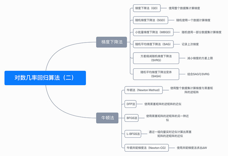
the original gradient descent algorithm, also known as Batch gradient descent/BGD, takes the whole data set as input to calculate the gradient.
$$ w=w-\eta \nabla_{w} \operatorname{Cost}(w) $$
the main disadvantage of this algorithm is that it uses the whole data set. When the data set is large, it may be abnormally time-consuming to calculate the gradient.
Stochastic Gradient Descent/SGD
each iteration update only randomly processes one data, not the whole data set.
$$ w=w-\eta \nabla_{w} \operatorname{Cost}\left(w, X_{i}, y_{i}\right) \quad i \in[1, N] $$
because the algorithm is a random data point, the cost function does not decline all the time, but fluctuates up and down. Adjusting the step size makes the result of the cost function decline as a whole, so the convergence rate does not decline as fast as the batch gradient.
Mini batch gradient descent / MBGD
the small batch gradient descent method combines the above two algorithms. When calculating the gradient, it uses neither the whole data set nor one data randomly selected at a time, but part of the data to update at a time.
$$ w=w-\eta \nabla_{w} \operatorname{Cost}\left(w, X_{(i: i+k)}, y_{(i: i+k)}\right) \quad i \in[1, N] $$
Random average gradient descent method1(Stochastic Average Gradient/SAG)
stochastic average gradient descent method is the optimization of stochastic gradient descent method. Due to the randomness of SGD, its convergence speed is slow. SAG records the gradient of the last position so that more information can be seen.
$$ \begin{aligned} w_{k+1} &=w_{k}-\frac{\eta}{N} \sum_{i=1}^{N}\left(d_{i}\right)_{k} \\ d_{k} &=\left\{\begin{array}{ll} \nabla_{w} \operatorname{Cost}\left(w_{k}, X_{i}, y_{i}\right) & i=i_{k} \\ d_{k-1} & i \neq i_{k} \end{array}\right. \end{aligned} $$
Variance reduction random gradient descent method2(Stochastic Variance Reduced Gradient/SVRG)
variance reduction stochastic gradient descent method is another optimization of stochastic gradient descent method. Because the convergence problem of SGD is that the variance of gradient is assumed to have an upper bound of constant, SVRG makes the convergence process more stable by reducing this variance.
$$ w_{k+1}=w_{k}-\eta\left(\nabla_{w} \operatorname{Cost}\left(w_{k}, X_{i}, y_{i}\right)-\nabla_{w} \operatorname{Cost}\left(\hat{w}, X_{i}, y_{i}\right)+\frac{1}{N} \sum_{j=1}^{N} \nabla_{w} \operatorname{Cost}\left(\hat{w}, X_{j}, y_{j}\right)\right) $$
Variation of random mean gradient descent method3(SAGA)
SAGA is the optimization of random average gradient descent method, which combines the variance reduction random gradient descent method.
$$ w_{k+1}=w_{k}-\eta\left(\nabla_{w} \operatorname{Cost}\left(w_{k}, X_{i}, y_{i}\right)-\nabla_{w} \operatorname{Cost}\left(w_{k-1}, X_{i}, y_{i}\right)+\frac{1}{N} \sum_{j=1}^{N} \nabla_{w} \operatorname{Cost}\left(w, X_{j}, y_{j}\right)\right) $$
3, Newton method
Newton Method
the original version of Newton's method takes the whole data set as input to calculate the gradient and Hesse matrix, and then calculate the falling direction
$$ w_{k+1}=w_{k}-\eta\left(H^{-1} \nabla_{w} \operatorname{Cost}\left(w_{k}\right)\right) $$
the main disadvantage of this algorithm is that it needs to find the Hesse matrix and its inverse matrix. When the dimension of x is too many, the process of finding the Hesse matrix will be extremely difficult.
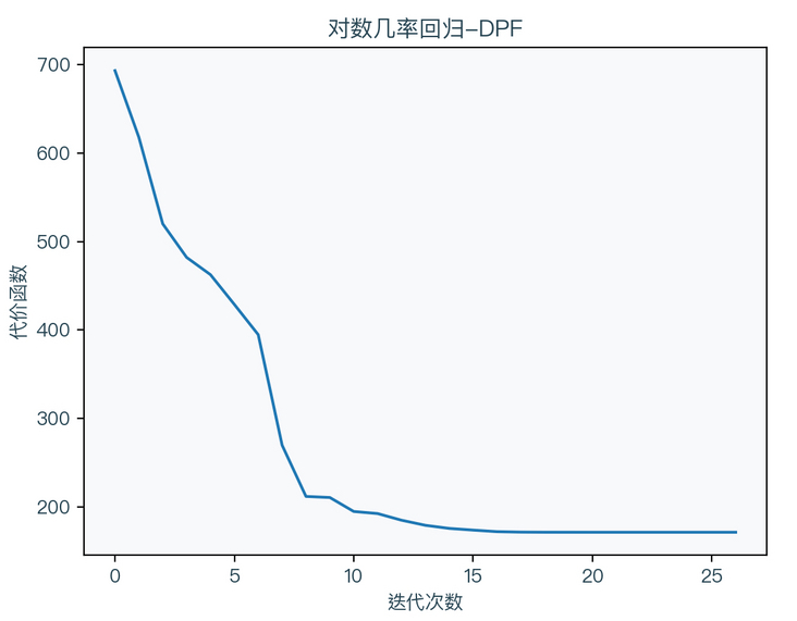
DFP method4(Davidon–Fletcher–Powell)
DFP method is a quasi Newton method. The algorithm is as follows:
$$ \begin{aligned} g_{k} &=\nabla_{w} \operatorname{Cost}\left(w_{k}\right) \\ d_{k} &=-D_{k} g_{k} \\ s_{k} &=\eta d_{k} \\ w_{k+1} &=w_{k}+s_{k} \\ g_{k+1} &=\nabla_{w} \operatorname{Cost}\left(w_{k+1}\right) \\ y_{k} &=g_{k+1}-g_{k} \\ D_{k+1} &=D_{k}+\frac{s_{k} s_{k}^{T}}{s_{k}^{T} y_{k}}-\frac{D_{k} y_{k} y_{k}^{T} D_{K}}{y_{k}^{T} D_{k} y_{k}} \end{aligned} $$
it can be seen that DFP no longer directly solves the Hessian matrix, but obtains the approximate value through iteration, where D is the approximation of the inverse matrix of the Hessian matrix.
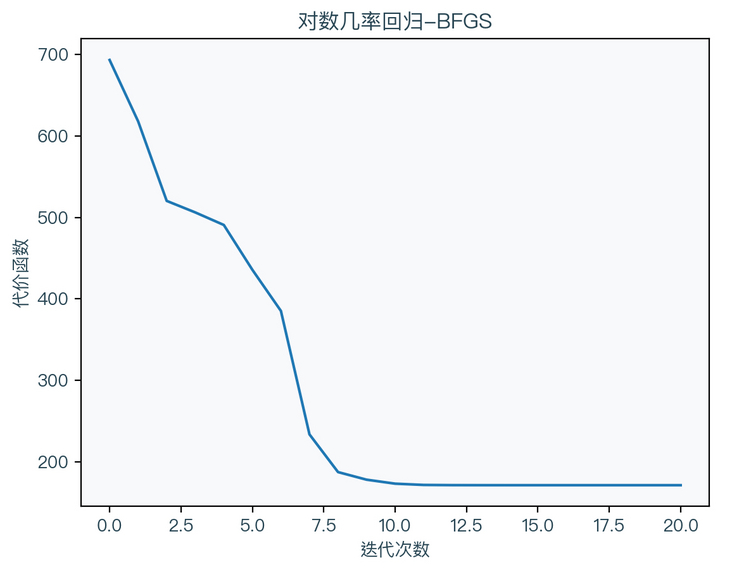
BFGS method5(Broyden–Fletcher–Goldfarb–Shanno)
The BFGS method as like as two peas Newton methods is basically the same as the DFP method.
$$ \begin{aligned} g_{k} &=\nabla_{w} \operatorname{Cost}\left(w_{k}\right) \\ d_{k} &=-D_{k} g_{k} \\ s_{k} &=\eta d_{k} \\ w_{k+1} &=w_{k}+s_{k+1} \\ g_{k+1} &=\nabla_{w} \operatorname{Cost}\left(w_{k+1}\right) \\ y_{k} &=g_{k+1}-g_{k} \\ D_{k+1} &=\left(I-\frac{s_{k} y_{k}^{T}}{y_{k}^{T} s_{k}}\right) D_{k}\left(I-\frac{y_{k} s_{k}^{T}}{y_{k}^{T} s_{k}}\right)+\frac{s_{k} s_{k}^{T}}{y_{k}^{T} s_{k}} \end{aligned} $$
it can be seen that the only difference between the BFGS method is the approximation method for the Hesse matrix, where D is the approximation of the inverse matrix of the Hesse matrix.
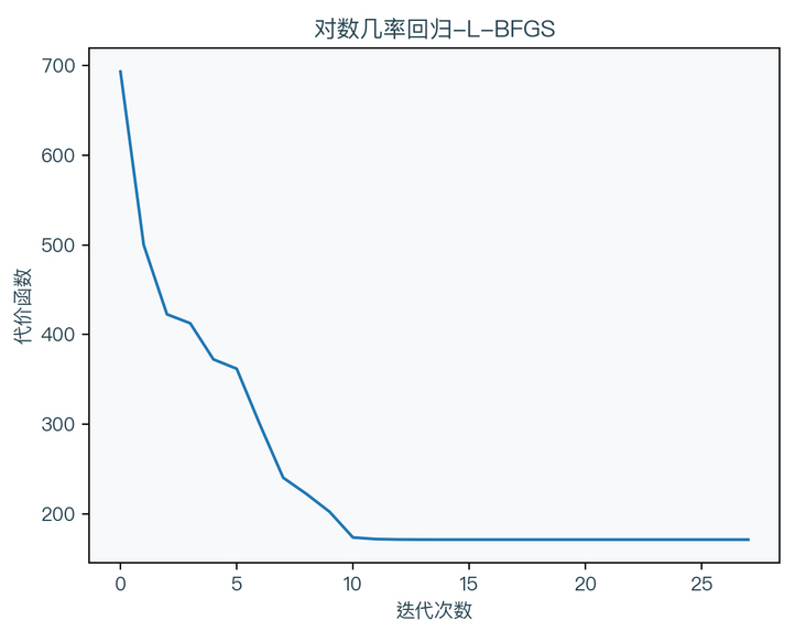
L-BFGS method6(Limited-memory Broyden–Fletcher–Goldfarb–Shanno)
because the BFGS method needs to store an approximate Hessian matrix, when the dimension of x is too large, the memory occupied by the Hessian matrix will be abnormally large. The L-BFGS method is another approximation of the BFGS method. The algorithm is as follows:
$$ \begin{aligned} g_{k} &=\nabla_{w} \operatorname{Cost}\left(w_{k}\right) \\ d_{k} &=-\operatorname{calcDirection}\left(s_{k-m: k-1}, y_{k-m: k-1}, \rho_{k-m: k-1}, g_{k}\right) \\ s_{k} &=\eta d_{k} \\ w_{k+1} &=w_{k}+s_{k} \\ g_{k+1} &=\nabla_{w} \operatorname{Cost}\left(w_{k+1}\right) \\ y_{k} &=g_{k+1}-g_{k} \\ \rho_{k} &=\frac{1}{y_{k}^{T} s_{k}} \end{aligned} $$
it can be seen that the L-BFGS method no longer directly saves the approximate Hessian matrix, but directly calculates it through a group of vectors when it is to be used, so as to save memory. The method of calculating the direction can refer to the implementation in the following code.
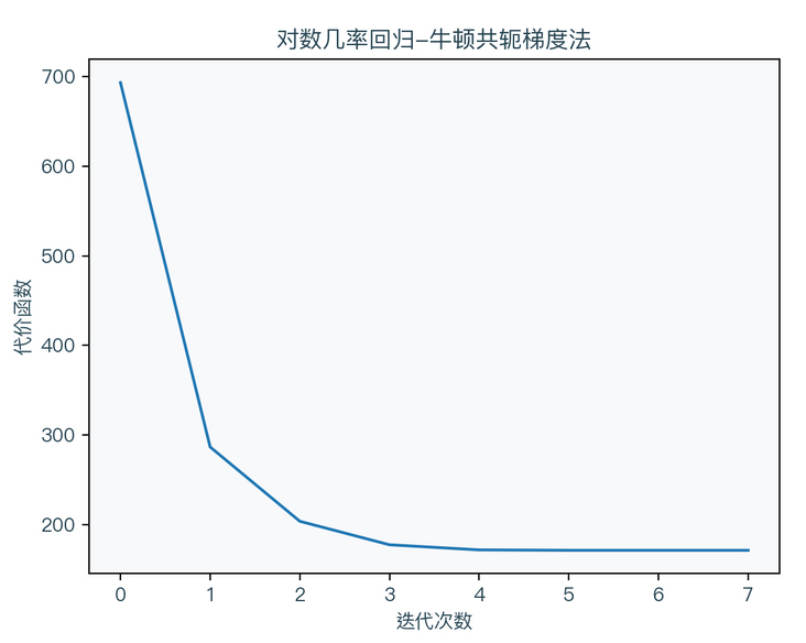
Newton conjugate gradient / Newton CG
Newton conjugate gradient method is the optimization of Newton method. The algorithm is as follows:
$$ \begin{aligned} g_{k} &=\nabla_{w} \operatorname{Cost}\left(w_{k}\right) \\ H_{k} &=\nabla_{w}^{2} \operatorname{Cost}\left(w_{k}\right) \\ \Delta w &=c g\left(g_{k}, H_{k}\right) \\ w_{k+1} &=w_{k}-\Delta w \end{aligned} $$
it can be seen that Newton's Conjugate Gradient method no longer solves the inverse matrix of Hesse matrix, but directly solves it through the Conjugate Gradient method Δ w. The Conjugate Gradient method is recommended in the references article 7. The principle and application of the algorithm are introduced in detail.
4, Code implementation
Use Python to implement the logarithmic probability regression algorithm (random gradient descent method):
import numpy as np

def logisticRegressionSGD(X, y, max_iter=100, tol=1e-4, step=1e-1):
   w = np.zeros(X.shape[1])
   xy = np.c_[X.reshape(X.shape[0], -1), y.reshape(X.shape[0], 1)]
   for it in range(max_iter):
       s = step / (np.sqrt(it + 1))
       np.random.shuffle(xy)
       X_new, y_new = xy[:, :-1], xy[:, -1:].ravel()
       for i in range(0, X.shape[0]):
           d = dcost(X_new[i], y_new[i], w)
           if (np.linalg.norm(d) <= tol):
               return w
           w = w - s * d
   return w
Use Python to implement the logarithmic probability regression algorithm (batch random gradient descent method):
import numpy as np

def logisticRegressionMBGD(X, y, batch_size=50, max_iter=100, tol=1e-4, step=1e-1):
    w = np.zeros(X.shape[1])
    xy = np.c_[X.reshape(X.shape[0], -1), y.reshape(X.shape[0], 1)]
    for it in range(max_iter):
        s = step / (np.sqrt(it + 1))
        np.random.shuffle(xy)
        for start in range(0, X.shape[0], batch_size):
            stop = start + batch_size
            X_batch, y_batch = xy[start:stop, :-1], xy[start:stop, -1:].ravel()
            d = dcost(X_batch, y_batch, w)
            if (np.linalg.norm(p_avg) <= tol):
                return w
            w = w - s * d
    return w
Use Python to implement the logarithmic probability regression algorithm (random average gradient descent method):
import numpy as np

def logisticRegressionSAG(X, y, max_iter=100, tol=1e-4, step=1e-1):
   w = np.zeros(X.shape[1])
   p = np.zeros(X.shape[1])
   d_prev = np.zeros(X.shape)
   for it in range(max_iter):
       s = step / (np.sqrt(it + 1))
       for it in range(X.shape[0]):
           i = np.random.randint(0, X.shape[0])
           d = dcost(X[i], y[i], w)
           p = p - d_prev[i] + d
           d_prev[i] = d
           p_avg = p / X.shape[0]
           if (np.linalg.norm(p_avg) <= tol):
               return w
           w = w - s * p_avg
   return w
Use Python to implement the logarithmic probability regression algorithm (variance reduction random gradient descent method):
import numpy as np

def logisticRegressionSVRG(X, y, max_iter=100, m = 100, tol=1e-4, step=1e-1):
    w = np.zeros(X.shape[1])
    for it in range(max_iter):
        s = step / (np.sqrt(it + 1))
        g = np.zeros(X.shape[1])
        for i in range(X.shape[0]):
            g = g + dcost(X[i], y[i], w)
        g = g / X.shape[0]
        tempw = w
        for it in range(m):
            i = np.random.randint(0, X.shape[0])
            d_tempw = dcost(X[i], y[i], tempw)
            d_w = dcost(X[i], y[i], w)
            d = d_tempw - d_w + g
            if (np.linalg.norm(d) <= tol):
                break
            tempw = tempw - s * d
        w = tempw
    return w
Implement logarithm probability regression algorithm (SAGA) using Python:
import numpy as np

def logisticRegressionSAGA(X, y, max_iter=100, tol=1e-4, step=1e-1):
   w = np.zeros(X.shape[1])
   p = np.zeros(X.shape[1])
   d_prev = np.zeros(X.shape)
   for i in range(X.shape[0]):
       d_prev[i] = dcost(X[i], y[i], w)
   for it in range(max_iter):
       s = step / (np.sqrt(it + 1))
       for it in range(X.shape[0]):
           i = np.random.randint(0, X.shape[0])
           d = dcost(X[i], y[i], w)
           p = d - d_prev[i] + np.mean(d_prev, axis=0)
           d_prev[i] = d
           if (np.linalg.norm(p) <= tol):
               return w
           w = w - s * p
   return w
Implement the logarithmic probability regression algorithm (DFP) using Python:
import numpy as np

def logisticRegressionDPF(X, y, max_iter=100, tol=1e-4):
   w = np.zeros(X.shape[1])
   D_k = np.eye(X.shape[1])
   g_k = dcost(X, y, w)
   for it in range(max_iter):
       d_k = -D_k.dot(g_k)
       s = lineSearch(X, y, w, d_k, 0, 10)
       s_k = s * d_k
       w = w + s_k
       g_k_1 = dcost(X, y, w)
       if (np.linalg.norm(g_k_1) <= tol):
           return w
       y_k = (g_k_1 - g_k).reshape(-1, 1)
       s_k = s_k.reshape(-1, 1)
       D_k = D_k + s_k.dot(s_k.T) / s_k.T.dot(y_k) - D_k.dot(y_k).dot(y_k.T).dot(D_k) / y_k.T.dot(D_k).dot(y_k)
       g_k = g_k_1
   return w
Implement the logarithmic probability regression algorithm (BFGS) using Python:
import numpy as np

def logisticRegressionBFGS(X, y, max_iter=100, tol=1e-4):
    w = np.zeros(X.shape[1])
    D_k = np.eye(X.shape[1])
    g_k = dcost(X, y, w)
    for it in range(max_iter):
        d_k = -D_k.dot(g_k)
        s = lineSearch(X, y, w, d_k, 0, 10)
        s_k = s * d_k
        w = w + s_k
        g_k_1 = dcost(X, y, w)
        if (np.linalg.norm(g_k_1) <= tol):
            return w
        y_k = (g_k_1 - g_k).reshape(-1, 1)
        s_k = s_k.reshape(-1, 1)
        a = s_k.dot(y_k.T)
        b = y_k.T.dot(s_k)
        c = s_k.dot(s_k.T)
        D_k = (np.eye(X.shape[1]) - a / b).dot(D_k).dot((np.eye(X.shape[1]) - a.T / b)) + c / b
        g_k = g_k_1
    return w
Implement the logarithmic probability regression algorithm (L-BFGS) using Python:
import numpy as np

def calcDirection(ss, ys, rhos, g_k, m, k):
    delta = 0
    L = k
    q = g_k.reshape(-1, 1)
    if k > m:
        delta = k - m
        L = m
    alphas = np.zeros(L)
    for i in range(L - 1, -1, -1):
        j = i + delta
        alpha = rhos[j].dot(ss[j].T).dot(q)
        alphas[i] = alpha
        q = q - alpha * ys[j]
    r = np.eye(g_k.shape[0]).dot(q)
    for i in range(0, L):
        j = i + delta
        beta = rhos[j].dot(ys[j].T).dot(r)
        r = r + (alphas[i] - beta) * ss[j]
    return -r.ravel()

def logisticRegressionLBFGS(X, y, m=100, max_iter=100, tol=1e-4):
    w = np.zeros(X.shape[1])
    g_k = dcost(X, y, w)
    d_k = -np.eye(X.shape[1]).dot(g_k)
    ss = []
    ys = []
    rhos = []
    for it in range(max_iter):
        d_k = calcDirection(ss, ys, rhos, g_k, m, it)
        s = lineSearch(X, y, w, d_k, 0, 1)
        s_k = s * d_k
        w = w + s_k
        g_k_1 = dcost(X, y, w)
        if (np.linalg.norm(g_k_1) <= tol):
            return w
        y_k = (g_k_1 - g_k).reshape(-1, 1)
        s_k = s_k.reshape(-1, 1)
        ss.append(s_k)
        ys.append(y_k)
        rhos.append(1 / (y_k.T.dot(s_k)))
        g_k = g_k_1
    return w
Implement the logarithmic probability regression algorithm (Newton conjugate gradient method) using Python:
import numpy as np

def cg(H, g, max_iter=100, tol=1e-4):
   """
   conjugate gradient method
   H * deltaw = g
   """
   deltaw = np.zeros(g.shape[0])
   i = 0
   r = g
   d = r
   delta = np.dot(r, r)
   delta_0 = delta
   while i < max_iter:
       q = H.dot(d)
       alpha = delta / (np.dot(d, q))
       deltaw = deltaw + alpha * d
       r = r - alpha * q
       delta_prev = delta
       delta = np.dot(r, r)
       if delta <= tol * tol * delta_0:
           break
       beta = delta / delta_prev
       d = r + beta * d
       i = i + 1
   return deltaw

def logisticRegressionNewtonCG(X, y, max_iter=100, tol=1e-4, step = 1.0):
   """
   Log probability regression using Newton conjugate gradient method( Newton-Conjugate Gradient)
   args:
       X - Training data set
       y - Target tag value
       max_iter - Maximum number of iterations
       tol - Tolerance value of variation
   return:
       w - weight coefficient
   """
   # Initialize w to zero vector
   w = np.zeros(X.shape[1])
   # Start iteration
   for it in range(max_iter):
       # Calculated gradient
       d = dcost(X, y, w)
       # When the gradient is small enough, end the iteration
       if np.linalg.norm(d) <= tol:
           break
       # Calculate Hesse matrix
       H = ddcost(X, y, w)
       # Calculated by conjugate gradient method Δ w
       deltaw = cg(H, d)
       w = w - step * deltaw
   return w
5, Third party library implementation
scikit-learn 8 realize logarithmic probability regression (random average gradient descent method):
from sklearn.linear_model import LogisticRegression

# Initialize log probability regressor, no regularization
reg = LogisticRegression(penalty="none", solver="sag")
# Fitting linear model
reg.fit(X, y)
# weight coefficient
w = reg.coef_
# intercept
b = reg.intercept_
scikit-learn 8 implement log probability regression (SAGA):
from sklearn.linear_model import LogisticRegression

# Initialize log probability regressor, no regularization
reg = LogisticRegression(penalty="none", solver="saga")
# Fitting linear model
reg.fit(X, y)
# weight coefficient
w = reg.coef_
# intercept
b = reg.intercept_
scikit-learn 8 log probability regression (L-BFGS):
from sklearn.linear_model import LogisticRegression

# Initialize log probability regressor, no regularization
reg = LogisticRegression(penalty="none", solver="lbfgs")
# Fitting linear model
reg.fit(X, y)
# weight coefficient
w = reg.coef_
# intercept
b = reg.intercept_
scikit-learn 8 realize logarithmic probability regression (Newton conjugate gradient method):
from sklearn.linear_model import LogisticRegression

# Initialize log probability regressor, no regularization
reg = LogisticRegression(penalty="none", solver="newton-cg")
# Fitting linear model
reg.fit(X, y)
# weight coefficient
w = reg.coef_
# intercept
b = reg.intercept_
7, Mind map
8, References
- https://hal.inria.fr/hal-0086...
- https://harkiratbehl.github.i...
- https://arxiv.org/pdf/1407.02...
- https://en.wikipedia.org/wiki...
- https://en.wikipedia.org/wiki...
- https://en.wikipedia.org/wiki...
- https://flat2010.github.io/20...
- https://scikit-learn.org/stab...
For a complete demonstration, please click here
Note: This article strives to be accurate and easy to understand, but as the author is also a beginner, his level is limited. If there are errors or omissions in the article, readers are urged to criticize and correct it by leaving a message
This article was first published in—— AI map , welcome to pay attention