In the previous section, we learned the KNN classification algorithm.Among them: Classification means that the Y variable is categorical, such as color category, computer brand, and reputation.

The linear regression algorithm learned today, where: Regression means that the Y variable is a continuous numerical variable, such as house price, population, and rainfall.

1. Simple linear regression

1-1, Simple Linear Regression

• Many decision-making processes are usually based on relationships between two or more variables
• Regression analysis is used to establish equations that simulate how two or more variables relate to each other.
• The predicted variable is called dependent variable, y, output
• Variables used to make predictions are called independent variables, x, input

1-2. Introduction of Simple Linear Regression

• Simple linear regression contains an independent variable (x) and a dependent variable (y)

• The relationship between the above two variables is simulated by a straight line

• If it contains more than two independent variables, it is called multiple regression.

1-3. Simple linear regression model

• The equation used to describe the relationship between dependent (y) and independent (X) variables and errors is called a regression model.

• Simple linear regression models are:

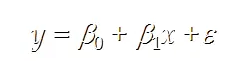
y: The predicted value of the sample, that is, the strain in the regression model

x: The characteristic value of the sample, that is, the independent variable in the regression model

Epsilon: An error term in a regression model that indicates variability contained in y but not explained by the linear relationship between x and Y

Essential: Find a straight line to best fit the relationship between sample characteristics and sample output markers

2. Derivation by Least Squares Method

ordinary

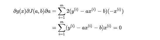
First, our goal is to find a and b so that the loss function:

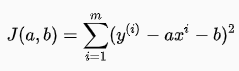
As small as possible.

Here, the simple linear problem is turned into an optimization problem.The following is the derivation of each position component of the function, where the derivative is 0 is the extreme value:

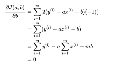
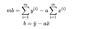
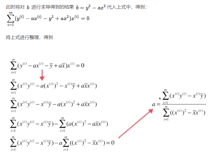
Then mb mentions before the equal sign, dividing both sides by m, and each item on the right side of the equal sign is equal to the mean.

This is much simpler to implement.

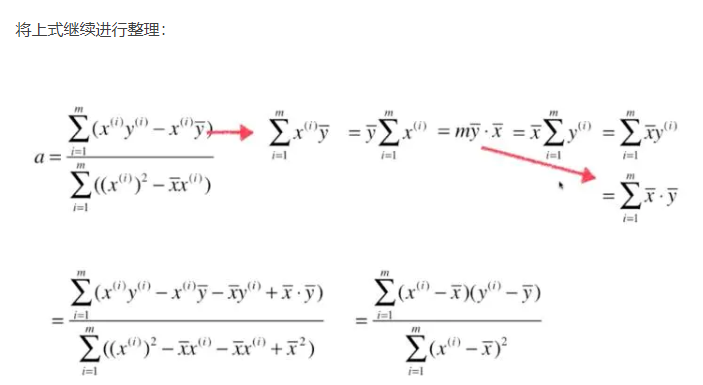
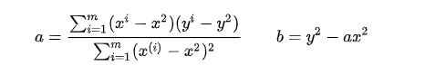
Finally, we get the expression of a and b by least squares:

vector

Bridging Style

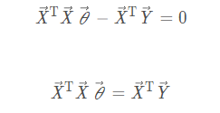
Change to Matrix Representation

Put Transpose Inside Brackets

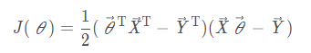
Multiplicative Expansion

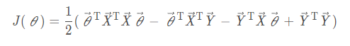
Finding gradients

Last Transpose Write On

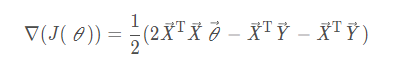
merge

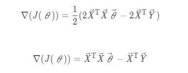
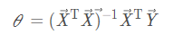
Find the stationary point of the gradient,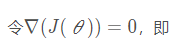

The final analytic formula for the parameter theta is obtained

Why not use least squares

In the last section, the least squares method is deduced theoretically and the result is very beautiful, but it is not often used in practice for the following reasons:

3. Implementation of Simple Linear Regression Code

Reference link: https://blog.csdn.net/zhaodedong/article/details/102855126

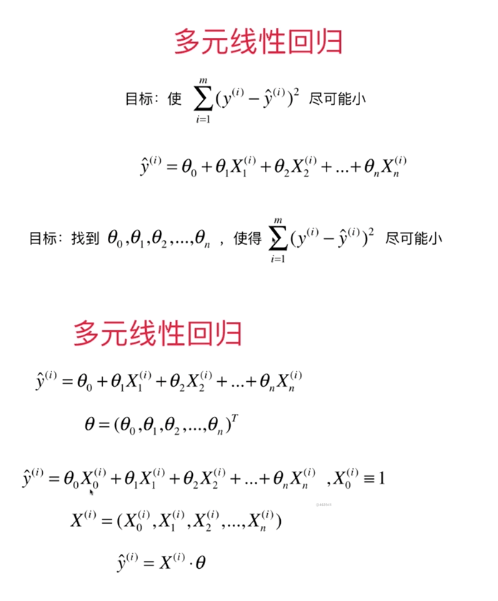
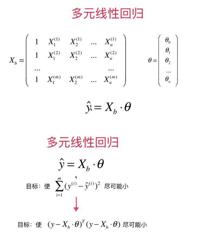
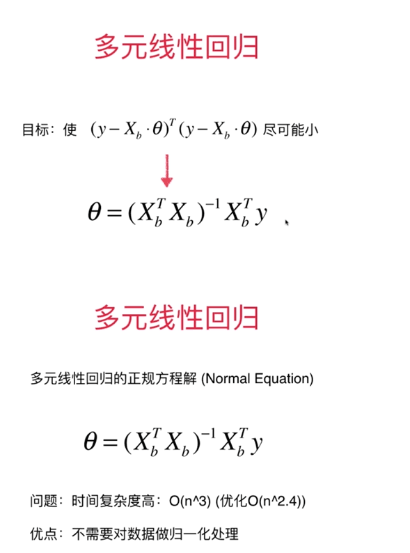
4. Multivariate Linear Regression

4-1. What is Multivariate Linear Regression

In regression analysis, if there are two or more independent variables, it is called multivariate regression.In fact, a phenomenon is often associated with multiple factors. Predicting or estimating a dependent variable by the optimal combination of multiple independent variables is more effective and practical than predicting or estimating it by only one independent variable.Therefore, multivariate linear regression is more practical than univariate linear regression.

4-2, Derivation

4-3, Code implementation

import numpy as np 
import matplotlib.pyplot as plt
from sklearn import datasets

#Loading datasets
boston=datasets.load_boston()
X = boston.data
y = boston.target
X = X[y < 50.0]
y = y[y < 50.0]


#Load your own modules
from playML.LinearRegression import LinearRegression
reg = LinearRegression()  #Instantiation process

reg.fit_normal(X_train,y_train) #The process of training datasets

reg.coef_ #View corresponding feature attribute values
'''
array([-1.18919477e-01,  3.63991462e-02, -3.56494193e-02,  5.66737830e-02,
	   -1.16195486e+01,  3.42022185e+00, -2.31470282e-02, -1.19509560e+00,
		2.59339091e-01, -1.40112724e-02, -8.36521175e-01,  7.92283639e-03,
	   -3.81966137e-01])
'''

reg.intercept_ #Intercept: 34.16143549624022

reg.score(x_test,y_test)  #View the accuracy of the algorithm: 0.8129802602658537  

Linear Regression Using sklearn

import numpy as np 
import matplotlib.pyplot as plt
from sklearn import datasets

#Loading data
boston=datasets.load_boston()

X = boston.data
y = boston.target

#Data preprocessing, removing points on the boundary
X = X[y < 50.0]
y = y[y < 50.0]

#The original data is divided into training data and test data by self-written segmentation method
from playML.model_selection import train_test_split
X_train,x_test,y_train,y_test=train_test_split(X,y,seed=666)

#Import corresponding modules
from sklearn.linear_model import LinearRegression
lin_reg = LinearRegression()
lin_reg.fit(X_train,y_train)

#Value of the eigenvalue
lin_reg.coef_

'''
array([-1.18919477e-01,  3.63991462e-02, -3.56494193e-02,  5.66737830e-02,
	   -1.16195486e+01,  3.42022185e+00, -2.31470282e-02, -1.19509560e+00,
		2.59339091e-01, -1.40112724e-02, -8.36521175e-01,  7.92283639e-03,
	   -3.81966137e-01])
'''

#intercept
lin_reg.intercept_  #34.16143549624665


#Test algorithm accuracy R Squared
lin_reg.score(x_test,y_test)  #0.8129802602658495