Catalog

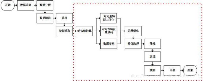
1. Overview of the process (this article is mainly the red box part)

2. Feature Processing Section

1. Overview

1.1 Some common questions

2. Specific treatment (see red box above for specific order)

2.1 Missing value handling (delete or fill)

2.2 Data format processing (data set partition, time format, etc.)

2.3 Data sampling (oversampled or undersampled, used when uneven)

2.4 Data preprocessing (converting original data to better format standard, normalized, binary)

2.5 Feature extraction (turn text into usable_dictionary, English, DNA,TF)

2.6 Dimension reduction (filtering (low variance, correlation coefficient), PCA)

2.7 Feature Project Example: Titanic Lifetime Analysis

3. Common SKlearn algorithms

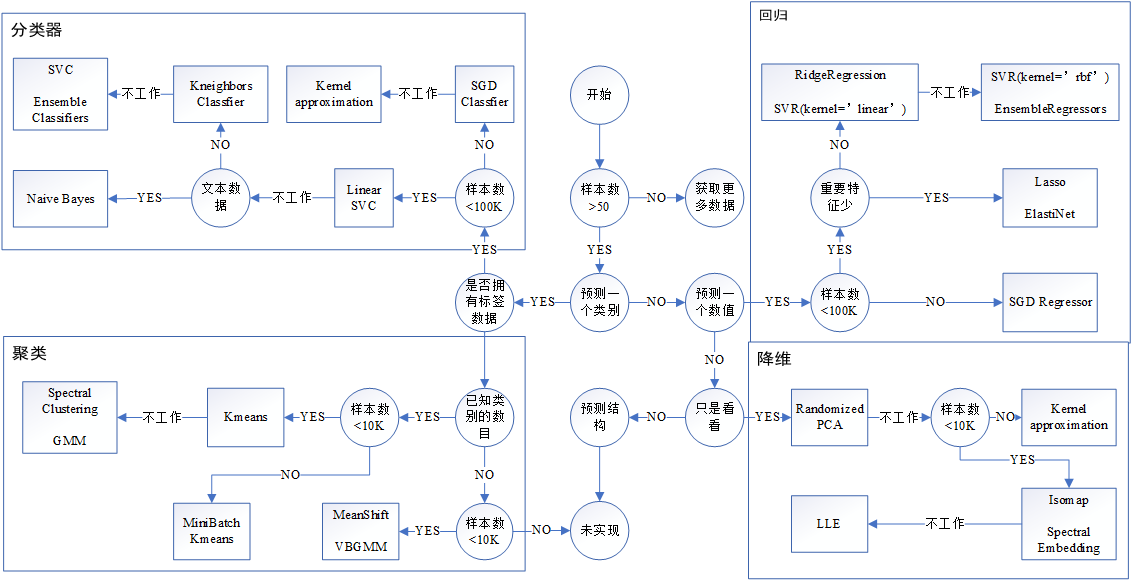
1. Decide what algorithm to use

2. Specific algorithm and its code

2.1 Classification Method (KNN, Logistic Regression, RF, Naive Bayesian, SVM)

2.2 Regression Method (KNN, Ridge Regression)

2.3 Clustering Method (K-means)

IV. Assessment

Refer to this article

5. Tuning

1. Try data and preprocessing first

2. Then select the model and adjust the model parameters

2.1 grid search

2.2 Random optimization methods (random trials)

2.3 Bayesian optimization method

2.4 Gradient-based optimization methods

2.5 Genetic algorithm (evolutionary optimization)

6. Some examples

1. Case: Predict facebook check-in location

2. Cases: 20 categories of news

3. Case Study: Boston House Price Forecast

4. Case: Cancer Classification Prediction - Benign/Malignant Breast Cancer Prediction

7. Model preservation and loading

1. Overview of the process (this article is mainly the red box part)

2. Feature Processing Section

Introduction: The main content of this section comes from
"Feature Engineering":A Nauseous Work--Deep Understanding of Feature Engineering_wx:wu805686220-CSDN Blog

Feature Engineering Introduction_Remote-CSDN Blog

1. Overview

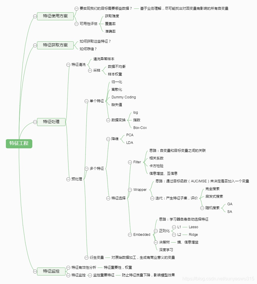
1.1 Some common questions

(1) There are missing values: missing values need to be supplemented (.dropna, etc.)
(2) Not in the same dimension: that is, the specifications of the features are different and cannot be compared together (standardized)
(3) Redundancy of information: some quantitative characteristics, such as interval division > If you only care about "passing" or "failing", then the score will be converted to "1" and "0" to indicate passing and failing (where > 60.)
(4) Qualitative features cannot be used directly: qualitative features need to be converted to quantitative features (such as one-hot, TF, etc.)
(5) Low information utilization: different machine learning

Algorithms and models differ in the use of information in data, so choose an appropriate model

2. Specific treatment (see red box above for specific order)

2.1 Missing value handling (delete or fill)

1) Delete missing values (dropna)

2) Filling in missing values: more commonly used, generally using the mean or majority
1 Fill with Fixed Values

A common method for missing eigenvalues is to fill them with fixed values, such as 0, -99, as in the case of -99 for this list of missing values

data['Column 1'] = data['Column 1'].fillna('-99')

(2) Fill in with mean

For numeric features, the missing values can also be filled with the mean of the missing data. Here, the missing values of the feature, gray scale, are filled with the mean.

data['Column 1'] = data['Column 1'].fillna(data['Column 1'].mean()))

(3) Fill in with the majority

Similar to the mean, missing values can be populated with a majority

data['Column 1'] = data['Column 1'].fillna(data['Column 1'].mode()))

Other fills such as interpolation, KNN,RF are detailed in the original blog

2.2 Data format processing (data set partition, time format, etc.)

1) Partition of datasets

Common datasets are divided into two parts:

• Training data: for training, building models
• Test data: Used during model validation to assess whether a model is valid

from sklearn.datasets import load_iris
from sklearn.model_selection import train_test_split

def datasets_demo():

    # Getting datasets
    iris = load_iris()
    print("Iris dataset:\n", iris)
    print("View the dataset description:\n", iris["DESCR"])
    print("View the name of the eigenvalue:\n", iris.feature_names)
    print("View eigenvalues:\n", iris.data, iris.data.shape)  # 150 samples

    # Dataset partition X as feature Y as label 
    """random_state Random number seeds, different seeds will result in different random sampling results"""
    x_train, x_test, y_train, y_test = train_test_split(iris.data, iris.target, test_size=0.2, random_state=22)

    return None

if __name__ == "__main__":
    datasets_demo()

2) Processing of time format (mainly converting to month, day, or day of the week, and then finding what you want)

* See details https://blog.csdn.net/kobeyu652453/article/details/108894807

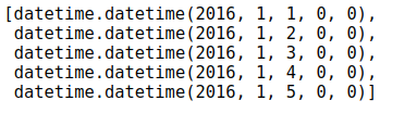
# Processing time data
import datetime

# Year, month, day
years = features['year']
months = features['month']
days = features['day']

# datetime format
dates = [str(int(year)) + '-' + str(int(month)) + '-' + str(int(day)) for year, month, day in zip(years, months, days)]
dates = [datetime.datetime.strptime(date, '%Y-%m-%d') for date in dates]
dates[:5]

                           

3) Tabular operations, merging or combining features

* See NP,PD tutorial for details

2.3 Data sampling (oversampled or undersampled, used when uneven)

_Oversampling of more categories/undersampling of fewer categories to balance distribution. Example: Credit card fraud, scam with too little data, use this time

def over_sample( y_origin, threshold):
    y = to_one_hot(y_origin, NUM_LABELS)
    y_counts = np.sum(y, axis=0)
    sample_ratio = threshold / y_counts * y
    sample_ratio = np.max(sample_ratio, axis=1)
    sample_ratio = np.maximum(sample_ratio, 1)
 
    index = ratio_sample(sample_ratio)
    # x_token_train = [x_token_train[i] for i in index]
 
    return y_origin[index]


def ratio_sample(ratio):
    sample_times = np.floor(ratio).astype(int)
 
    # random sample ratio < 1 (decimal part)
    sample_ratio = ratio - sample_times
    random = np.random.uniform(size=sample_ratio.shape)
    index = np.where(sample_ratio > random)
    index = index[0].tolist()
 
    # over sample fixed integer times
    row_num = sample_times.shape[0]
    for row_index, times in zip(range(row_num), sample_times):
        index.extend(itertools.repeat(row_index, times))
 
    return index

2.4 Data preprocessing (converting original data to better format standard, normalized, binary)

The main conversion methods are the following (the first four commonly used):

1) Standardization (very common)

Used for: data gaps between features are particularly large (e.g., deposit amounts and the number of neighborhoods around the bank, not on a scale)

from sklearn.preprocessing import StandardScaler
#Standardized, returned values are standardized data
StandardScaler().fit_transform(iris.data)

2) Normalization

Meaning: Sample vectors are converted into "unit vectors" when similarity is calculated by point multiplication or other kernel functions.

Under what circumstances (no) normalization is required:

• Need: Parameter-based models or distance-based models are all feature normalization.
• No: Tree-based methods do not require normalization of features, such as random forests, bagging s, boosting s, and so on.

from sklearn.preprocessing import Normalizer
#Normalized, returned value is normalized data
Normalizer().fit_transform(iris.data)

3) Binarization (>60 pass, marked 1)

With where or Binarizer

from sklearn.preprocessing import Binarizer
 #Binary, threshold set to 3, return value to binary data
Binarizer(threshold=3).fit_transform(iris.data)

Other: Zoom in and out, just look at the text

2.5 Feature extraction (turn text into usable_dictionary, English, DNA,TF)

1) Dictionary feature extraction: (Dictionary to Matrix)

from sklearn.feature_extraction import DictVectorizer

def dict_demo():

    data = [{'city':'Beijing', 'temperature':100},
            {'city':'Shanghai', 'temperature':60},
            {'city':'Shenzhen', 'temperature':30}]

    # 1. Instantiate a converter class
    #transfer = DictVectorizer() # Return sparse matrix
    transfer = DictVectorizer(sparse=False)

    # 2. Call fit_transform()
    data_new = transfer.fit_transform(data)
    print("data_new: \n", data_new)   # Transformed
    print("Feature name:\n", transfer.get_feature_names())

    return None

if __name__ == "__main__":
    dict_demo()

Result:

data_new: 
 [[  0.   1.   0. 100.]
 [  1.   0.   0.  60.]
 [  0.   0.   1.  30.]]
 Feature name:
 ['city=Shanghai', 'city=Beijing', 'city=Shenzhen', 'temperature']

2) Text Feature Extraction (Text to Matrix)

Applying 1. Chinese and English word segmentation, then switching to matrix 2. DNA SEQS processing, bag model

2.1) English text participle

from sklearn.feature_extraction.text import CountVectorizer

def count_demo():

    data = ['life is short,i like like python',
            'life is too long,i dislike python']

    # 1. Instantiate a converter class
    transfer = CountVectorizer()
    #Here's another stop_word(), which is the word to stop at
    transfer1 = CountVectorizer(stop_words=['is', 'too'])

    # 2. Call fit_transform
    data_new = transfer.fit_transform(data)
    print("data_new: \n", data_new.toarray())  # toarray to a two-dimensional array
    print("Feature name:\n", transfer.get_feature_names())

    return None


if __name__ == "__main__":
    count_demo()

Result

data_new: 
 [[0 1 1 2 0 1 1 0]
 [1 1 1 0 1 1 0 1]]
Feature name:
 ['dislike', 'is', 'life', 'like', 'long', 'python', 'short', 'too']

2.2) Chinese word breakers

from sklearn.feature_extraction.text import CountVectorizer
import jieba


def count_chinese_demo2():
 
    data = ['One is that today is cruel, tomorrow is cruel and the day after tomorrow is beautiful, but most of them die tomorrow evening, so everyone should not give up today.',
            'We see light coming from distant galaxies millions of years ago, so when we see the universe, we are looking at its past.',
            'If he knows something in only one way, he won't really know it. The secret to knowing what it really means depends on how it relates to what we know.']

    data_new = []
    for sent in data:
        data_new.append(cut_word(sent))
    print(data_new)

    1,Instantiate a converter class(Call People
    transfer = CountVectorizer()

    2,call fit_transform(work
    data_final = transfer.fit_transform(data_new)
    print("data_final:\n", data_final.toarray())
    print("Feature name:\n", transfer.get_feature_names())

    return None


def cut_word(text):
    """
    Make a Chinese participle: "I love Tian'anmen in Beijing" -> "I love Tian'anmen, Beijing"
    """
    return ' '.join(jieba.cut(text))


if __name__ == "__main__":
    count_chinese_demo2()
    #print(cut_word('I love Tian'anmen in Beijing'))

2.3) Tf-idf Text Feature Extraction: Find Important Words and Convert to Matrix

from sklearn.feature_extraction.text import CountVectorizer, TfidfVectorizer
import jieba

def tfidf_demo():
    """
    use TF-IDF Method for text feature extraction
    """
    data = ['One is that today is cruel, tomorrow is cruel and the day after tomorrow is beautiful, but most of them die tomorrow evening, so everyone should not give up today.',
            'We see light coming from distant galaxies millions of years ago, so when we see the universe, we are looking at its past.',
            'If he knows something in only one way, he won't really know it. The secret to knowing what it really means depends on how it relates to what we know.']

    data_new = []
    for sent in data:
        data_new.append(cut_word(sent))
    print(data_new)

    1,Instantiate a converter class
    transfer = TfidfVectorizer()

    2,call fit_transform
    data_final = transfer.fit_transform(data_new)
    print("data_final:\n", data_final.toarray())
    print("Feature name:\n", transfer.get_feature_names())
    return None


def cut_word(text):
    """
    Make a Chinese participle: "I love Tian'anmen in Beijing" -> "I love Tian'anmen, Beijing"
    """
    return ' '.join(jieba.cut(text))



if __name__ == "__main__":
    tfidf_demo()
    #print(cut_word('I love Tian'anmen in Beijing'))

Result:

['One is that today is cruel, tomorrow is cruel and the day after tomorrow is beautiful, but most of them die tomorrow evening, so everyone should not give up today.', 'We see light coming from distant galaxies millions of years ago, so when we see the universe, we are looking at its past.', 'If he knows something in only one way, he won't really know it. The secret to knowing what it really means depends on how it relates to what we know.']
data_final:
 [[0.30847454 0.         0.20280347 0.         0.         0.
  0.40560694 0.         0.         0.         0.         0.
  0.20280347 0.         0.20280347 0.         0.         0.
  0.         0.20280347 0.20280347 0.         0.40560694 0.
  0.20280347 0.         0.40560694 0.20280347 0.         0.
  0.         0.20280347 0.20280347 0.         0.         0.20280347
  0.        ]
 [0.         0.         0.         0.2410822  0.         0.
  0.         0.2410822  0.2410822  0.2410822  0.         0.
  0.         0.         0.         0.         0.         0.2410822
  0.55004769 0.         0.         0.         0.         0.2410822
  0.         0.         0.         0.         0.48216441 0.
  0.         0.         0.         0.         0.2410822  0.
  0.2410822 ]
 [0.12826533 0.16865349 0.         0.         0.67461397 0.33730698
  0.         0.         0.         0.         0.16865349 0.16865349
  0.         0.16865349 0.         0.16865349 0.16865349 0.
  0.12826533 0.         0.         0.16865349 0.         0.
  0.         0.16865349 0.         0.         0.         0.33730698
  0.16865349 0.         0.         0.16865349 0.         0.
  0.        ]]

Feature name:
['one kind', 'Can't,', 'No', 'before', 'understand', 'Thing', 'Today', 'Light is in', 'Millions of years', 'Issue', 'Depending on', 'only need', 'The day after tomorrow', 'Meaning', 'Gross', 'How', 'If', 'universe', 'We', 'therefore', 'give up', 'mode', 'Tomorrow', 'Galaxy', 'Night', 'Something', 'cruel', 'each', 'notice', 'real', 'Secret', 'Absolutely', 'fine', 'contact', 'Past times', 'still', 'such']

2.4) DNA SEQS treatment

1.First put seqs Data Cutting,6 A set of bases

def Kmers_funct(seq, size=6):
    return [seq[x:x+size] for x in range(len(seq) - size + 1)]

2.Reuse CountVectorizer
from sklearn.feature_extraction.text import CountVectorizer
cv = CountVectorizer(ngram_range=(4,4))
X = cv.fit_transform(textsList)

3.Conversion complete, training lost

2.6 Dimension reduction (filtering (low variance, correlation coefficient), PCA)

What do you mean: The process of reducing the number of random variables (characteristics) to get a set of primary variables (that is, to reduce the number of training columns)

1) Feature selection (find out important features from original features differences between human and dog: skin, height)

First: Low variance filtering (discard unimportant)

from sklearn.feature_selection import VarianceThreshold


def variance_demo():
    """
    Low variance feature filtering
    """

    # 1. Getting data
    data = pd.read_csv('factor_returns.csv')
    print('data:\n', data)
    data = data.iloc[:,1:-2]
    print('data:\n', data)

    # 2. Instantiate a converter class
    #transform = VarianceThreshold()
    transform = VarianceThreshold(threshold=10)

    # 3. Call fit_transform
    data_new = transform.fit_transform(data)
    print("data_new\n", data_new, data_new.shape)

    return None

if __name__ == "__main__":
    variance_demo()

Second: correlation coefficients (which are also trivial to discard, but are judged by correlation coefficients)

from sklearn.feature_selection import VarianceThreshold
from scipy.stats import pearsonr

def variance_demo():
    """
    Low variance feature filter correlation coefficient
    """

    # 1. Getting data
    data = pd.read_csv('factor_returns.csv')
    print('data:\n', data)
    data = data.iloc[:,1:-2]
    print('data:\n', data)

    # 2. Instantiate a converter class
    transform = VarianceThreshold()
    transform1 = VarianceThreshold(threshold=10)

    # 3. Call fit_transform
    data_new = transform.fit_transform(data)
    print("data_new\n", data_new, data_new.shape)

    # Calculate the correlation coefficient between two variables
    r = pearsonr(data["pe_ratio"],data["pb_ratio"])
    print("Coefficient of correlation:\n", r)
    return None


if __name__ == "__main__":
    variance_demo()

2)PCA

Notice mainly n_compnents: decimal indicating how much information is retained, integer how many features are reduced

from sklearn.decomposition import PCA

def pca_demo():
    """
    PCA dimensionality reduction
    """

    data = [[2,8,4,5], [6,3,0,8], [5,4,9,1]]

    # 1. Instantiate a converter class
    transform = PCA(n_components=2)  # Four features down to two

    # 2. Call fit_transform
    data_new = transform.fit_transform(data)
    print("data_new\n", data_new)

    transform2 = PCA(n_components=0.95)  # Keep 95% of the information

    data_new2 = transform2.fit_transform(data)
    print("data_new2\n", data_new2)

    return None

if __name__ == "__main__":
    pca_demo()

2.7 Feature Project Example: Titanic Lifetime Analysis

The above parts are commonly used by me (I compare dishes). I can see the original text in other ways.

Below is the case code

import pandas as pd

1,get data
path = "C:/DataSets/titanic.csv"
titanic = pd.read_csv(path) #1313 rows × 11 columns

# Screening Eigenvalues and Target Values
x = titanic[["pclass", "age", "sex"]]
y = titanic["survived"]

2,data processing
# 1) Treatment of missing values
x["age"].fillna(x["age"].mean(), inplace=True)

# 2) Convert to Dictionary
x = x.to_dict(orient="records")


3,Data Set Partitioning
from sklearn.model_selection import train_test_split
x_train, x_test, y_train, y_test = train_test_split(x, y, random_state=22)


4,Yes x_train,test Dictionary Feature Extraction
from sklearn.feature_extraction import DictVectorizer
transfer = DictVectorizer()
x_train = transfer.fit_transform(x_train)
x_test = transfer.transform(x_test)


5.Decision Tree Estimator
from sklearn.tree import DecisionTreeClassifier, export_graphviz
estimator = DecisionTreeClassifier(criterion='entropy')
estimator.fit(x_train, y_train)

6.Model evaluation
y_predict = estimator.predict(x_test)
print("y_predict:\n", y_predict)
print("Direct required read true and predicted values:\n", y_test == y_predict)  # Direct comparison

# Method 2: Calculate the accuracy
score = estimator.score(x_test, y_test)  # Eigenvalues of Test Sets, Target Values of Test Sets
print("Accuracy:", score)

# Visual Decision Tree (not required)
export_graphviz(estimator, out_file='titanic_tree.dot', feature_names=transfer.get_feature_names())

import matplotlib.pyplot as plt
from sklearn.tree import plot_tree
plot_tree(decision_tree=estimator)
plt.show()

3. Common SKlearn algorithms

The main content of this article comes from 9 common algorithms for machine learning _Superior De Five-CSDN Blog _Common algorithms for machine learning

1. Decide what algorithm to use

2. Specific algorithm and its code

They are basically four steps: guide (from...), modeling (knn=...), training and prediction (.fit(). predict()).

2.1 Classification Method (KNN, Logistic Regression, RF, Naive Bayesian, SVM)

2.1.1 KNN (regression, classification available)

Introduction:
The k Nearest Neighbor Classification (KNN) algorithm finds the k records closest to the new data from the training set and determines the category of the new data based on their main classification.
The algorithm involves three main points: training set, distance or similar measurement, and k size.

Advantages: Suitable for multiple classification problems

Simple, easy to understand, easy to implement, no parameter estimation, no training required

Suitable for classifying rare events (e.g., constructing loss prediction models when the loss rate is very low, e.g. less than 0.5%)

It is particularly suitable for multi-classification problems (objects with multiple class labels), such as functional classification based on genetic characteristics, where kNN performs better than SVM.

Disadvantages: High memory overhead, slower

Lazy algorithm, large amount of calculation, large memory overhead and slow score when classifying test samples

It is poorly interpretable and cannot give rules like decision trees.

Implementation code:

1.Import:

Classification issues:
from sklearn.neighbors import KNeighborsClassifier
 Regression problems:
from sklearn.neighbors import KNeighborsRegressor

2.Create a model
KNC = KNeighborsClassifier(n_neighbors=5)
KNR = KNeighborsRegressor(n_neighbors=3)

3.train
KNC.fit(X_train,y_train)
KNR.fit(X_train,y_train)

4.Forecast
y_pre = KNC.predict(x_test)
y_pre = KNR.predict(x_test)

2.1.2 Logistic Regression (logiscic):

Introduction: Can be seen as a more accurate linear regression

The main idea of using logistic regression to classify is to establish regression formulas for classifying boundary lines based on existing data, in which the term "regression" derives from the best fit, which means to find the best set of fitting parameters.

The practice of training classifiers is to find the best fitting parameters, using the optimal algorithm. Next, the mathematical principle of this binary output classifier is introduced.

Code:

1.Import
from sklearn.linear_model import LogisticRegression

2.Create a model
logistic = LogisticRegression(solver='lbfgs')

notes:solver Selection of parameters:
"liblinear": Small-scale datasets    <5~10k
"lbfgs", "sag" or "newton-cg": Large-scale datasets and multi-classification problems <30k
"sag": Extremely large datasets >30k


3.train
logistic.fit(x_train,y_train)

4.Forecast
y_pre = logistic.predict(x_train,y_train)

        

2.1.3 Random forests (very common)

    from sklearn.datasets import load_iris
    from sklearn.ensemble import RandomForestClassifier
    import pandas as pd
    import numpy as np
     
    iris = load_iris()
    df = pd.DataFrame(iris.data, columns=iris.feature_names)
    df['is_train'] = np.random.uniform(0, 1, len(df)) <= .75
    df['species'] = pd.Factor(iris.target, iris.target_names)
    df.head()
     
    train, test = df[df['is_train']==True], df[df['is_train']==False]
     
    features = df.columns[:4]
    clf = RandomForestClassifier(n_jobs=2)
    y, _ = pd.factorize(train['species'])
    clf.fit(train[features], y)
     
    preds = iris.target_names[clf.predict(test[features])]
    pd.crosstab(test['species'], preds, rownames=['actual'], colnames=['preds'])

Short version:

# Import algorithm
from sklearn.ensemble import RandomForestRegressor

# modeling
rf = RandomForestRegressor(n_estimators= 1000, random_state=42)

# train
rf.fit(train_features, train_labels)

# Forecast
y_pre=rf.predict(test_features)

2.1.4 Naive Bayes

Introduction: Simple Bayesian is Bayesian when variables are independent of each other. Don't be frightened by name

• 1. Gaussian (normal) distribution Naive Bayesian

• For general classification problems

• Use:

  1.Import
  from sklearn.naive_bayes import GaussianNB
  
  2.Create a model
  gNB = GaussianNB()
  
  3.train
  gNB.fit(data,target)
  
  4.Forecast
  y_pre = gNB.predict(x_test)

  2. Polynomial distribution Naive Bayesian (there is also a Bernoulli distribution. Similar to this, used in small quantities)

  • Suitable for text data (features represent times, such as the number of occurrences of a word)
  • DNA sequences can be used as features (actually text, just AGCT)
  • Commonly used for multi-classification problems

• Use

  1.Import
  from sklearn.naive_bayes import MultinomialNB
  
  2.Create a model
  mNB = MultinomialNB()
  
  3.Convert Character Set to Frequency
  from sklearn.feature_extraction.text import TfidfVectorizer
  
  #Build Tf objects first (what is Tf above)
  tf = TfidfVectorizer()
  #Train tf objects using datasets and label sets to convert
  tf.fit(X_train,y_train)
  #Text Set---->Word Frequency Set
  X_train_tf = tf.transform(X_train)
  
  4.Using word frequency set to train machine learning model
  mNB.fit(X_train_tf,y_train)
  
  5.Forecast
  
  #Convert Character Set to Word Frequency Set
  x_test = tf.transform(test_str)
  
  #Forecast
  mNB.predict(x_test)
  
  

2.1.5 Support Vector Machine SVM

Introduction: The idea of SVM is to find the nearest point from the hyperplane and find the optimal solution through its constraints.

Use

1.Import
 Handle classification issues:
from sklearn.svm import SVC
 Handling regression issues:
from sklearn.svm import SVR

2.Create a model (used in regression) SVR)
svc = SVC(kernel='linear')
svc = SVC(kernel='rbf')
svc = SVC(kernel='poly')

3.train
svc_linear.fit(X_train,y_train)
svc_rbf.fit(X_train,y_train)
svc_poly.fit(X_train,y_train)

4.Forecast
linear_y_ = svc_linear.predict(x_test)
rbf_y_ = svc_rbf.predict(x_test)
poly_y_ = svc_poly.predict(x_test)

2.2 Regression Method (KNN, Ridge Regression)

2.2.1 KNN (same as above)

Ridge regression

Introduction: The improved least squares method with linear regression to avoid over-fitting and under-fitting to some extent

#1. Import
from sklearn.linear_model import Ridge

#2. Create a model
# alpha is the reduction factor lambda, you can try the effect with your own dichotomy
# If alpha is set to zero, it is a normal linear regression
ridge = Ridge(alpha=0)

#3. Training
ridge.fit(data,target)

#4. Forecast
target_pre = ridge.predict(target_test)

2.2.3lasso regression

2.2.4RF (same as above)

2.2.5 Support Vector Machine SVM (same as above)

2.3 Clustering Method (K-means)

K-means (unsupervised learning)

principle

• The concept of clustering: an unsupervised learning that automatically groups similar objects into the same cluster without knowing the category beforehand.
• The K-Means algorithm is a clustering analysis algorithm. It mainly calculates the data aggregation algorithm by continuously taking the nearest mean from the seed point.

Code:

1.Import
from sklearn.cluster import KMeans

2.Create a model
# Building Machine Learning Objects kemans, specifying the number of classifications
kmean = KMeans(n_clusters=2)

3.Training data
# Note: Clustering algorithms do not have y_train
kmean.fit(X_train)

4.Forecast data
y_pre = kmean.predict(X_train)

IV. Assessment

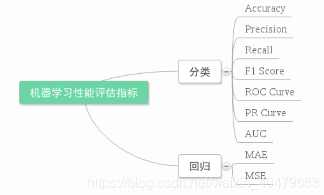
Refer to this article

Code Summary for Machine Learning Training Modeling, Integrated Model, Model Evaluation (Update 2019.05.21)_Dumb Generation Ma-CSDN Blog

5. Tuning

1. Try data and preprocessing first

Prioritize data itself and preprocessing, and work on Feature Engineering (choose more distinct features, clean data, compression, etc.)

2. Then select the model and adjust the model parameters

2.1 grid search

Introduction: Grid search is a violent method of tuning parameters by traversing all possible parameter values to get the best combination of all parameter combinations. (Just a parameter test)

Code:

#y = data['diagnosis']
#x = data.drop(['id','diagnosis','Unnamed: 32'],axis =1)

from sklearn.model_selection import train_test_split,GridSearchCV
#from sklearn.pipeline import Pipeline
#from sklearn.linear_model import LogisticRegression
#from sklearn.preprocessing import StandardScaler

#train_X,val_X,train_y,val_y = train_test_split(x,y,test_size=0.2,random_state=1)
pipe_lr = Pipeline([('scl',StandardScaler()),('clf',LogisticRegression(random_state=0))])

param_range=[0.0001,0.001,0.01,0.1,1,10,100,1000] What number to try
param_penalty=['l1','l2']
param_grid=[{'clf__C':param_range,'clf__penalty':param_penalty}]

gs = GridSearchCV(estimator=pipe_lr,
                 param_grid=param_grid,
                 scoring='f1',
                 cv=10,
                 n_jobs=-1)
gs = gs.fit(train_X,train_y)

print(gs.best_score_)
print(gs.best_params_)

2.2 Random optimization methods (random trials)

Code:

from sklearn.datasets import load_iris
from sklearn.ensemble import RandomForestRegressor
iris = load_iris()
rf = RandomForestRegressor(random_state = 42)
from sklearn.model_selection import RandomizedSearchCV
random_grid = {'n_estimators': n_estimators,
               'max_features': max_features,
               'max_depth': max_depth,
               'min_samples_split': min_samples_split,
               'min_samples_leaf': min_samples_leaf,
               'bootstrap': bootstrap}
rf_random = RandomizedSearchCV(estimator = rf, param_distributions = random_grid, n_iter = 100, cv = 3, verbose=2, random_state=42, n_jobs = -1)# Fit the random search model

rf_random.fit(X,y)

#print the best score throughout the grid search
print rf_random.best_score_
#print the best parameter used for the highest score of the model.
print rf_random.best_param_

The following three types do not have fixed code, depending on the specific project needs

2.3 Bayesian optimization method

2.4 Gradient-based optimization methods

2.5 Genetic algorithm (evolutionary optimization)

6. Some examples

1. Case: Predict facebook check-in location

Process analysis:
1) Get data
2) Data Processing
Purpose:

• Eigenvalue x:2<x<2.5
• Target y:1.0<y<1.5
• Time ->Years, Days, Hours and Seconds
• Filter places with fewer check-ins
  3) Feature Engineering: Standardization
  4) KNN algorithm prediction process
  5) Model Selection and Optimization
  6) Model evaluation

  import pandas as pd
  # 1. Getting data
  data = pd.read_csv("./FBlocation/train.csv") #29118021 rows × 6 columns
  
  # 2. Basic Data Processing
  # 1) Reduce data range
  data = data.query("x<2.5 & x>2 & y<1.5 & y>1.0") #83197 rows × 6 columns
  # 2) Processing time characteristics
  time_value = pd.to_datetime(data["time"], unit="s") #Name: time, Length: 83197
  date = pd.DatetimeIndex(time_value)
  data["day"] = date.day
  data["weekday"] = date.weekday
  data["hour"] = date.hour
  data.head() #83197 rows × 9 columns
  # 3) Filter places with fewer check-ins
  place_count = data.groupby("place_id").count()["row_id"]  #2514 rows × 8 columns
  place_count[place_count > 3].head()
  data_final = data[data["place_id"].isin(place_count[place_count>3].index.values)]
  data_final.head() #80910 rows × 9 columns
  
  # Screening Eigenvalues and Target Values
  x = data_final[["x", "y", "accuracy", "day", "weekday", "hour"]]
  y = data_final["place_id"]
  
  # Data Set Partitioning
  from sklearn.model_selection import train_test_split
  x_train, x_test, y_train, y_test = train_test_split(x, y)
  
  from sklearn.preprocessing import StandardScaler
  from sklearn.neighbors import KNeighborsClassifier
  from sklearn.model_selection import GridSearchCV
  
  # 3. Feature Engineering: Standardization
  transfer = StandardScaler()
  x_train = transfer.fit_transform(x_train)  # Standardization of training sets
  x_test = transfer.transform(x_test)        # Test Set Standardization
  
  # 4. KNN algorithm predictor
  estimator = KNeighborsClassifier()
  # Join Grid Search and Cross Validation
  # Parameter preparation
  param_dict = {"n_neighbors": [3,5,7,9]}
  estimator = GridSearchCV(estimator, param_grid=param_dict, cv=5)  # 10% discount, small amount of data, you can fold more
  
  estimator.fit(x_train, y_train)
  
  # 5. Model Evaluation
  # Method 1: Direct comparison of true and predicted values
  y_predict = estimator.predict(x_test)
  print("y_predict:\n", y_predict)
  print("Direct required read true and predicted values:\n", y_test == y_predict)  # Direct comparison
  
  # Method 2: Calculate the accuracy
  score = estimator.score(x_test, y_test)  # Eigenvalues of Test Sets, Target Values of Test Sets
  print("Accuracy:", score)
  
  # View the best parameters: best_params_
  print("Optimal parameters:", estimator.best_params_)
  # Best result: best_score_
  print("Best results:", estimator.best_score_)
  # Best estimator: best_estimator_
  print("Best estimator:", estimator.best_estimator_)
  # Cross-validation results: cv_results_
  print("Cross-validation results:", estimator.cv_results_)
  

  2. Cases: 20 categories of news

  Step 1 Analysis
  1) Get data
  2) Partitioning datasets
  3) Feature Engineering: Text Feature Extraction
  4) Naive Bayesian predictor process
  5) Model evaluation

2 Specific Code

from sklearn.model_selection import train_test_split    # Partition Dataset
from sklearn.datasets import fetch_20newsgroups
from sklearn.feature_extraction.text import TfidfVectorizer  # Text Feature Extraction
from sklearn.naive_bayes import MultinomialNB           # Naive Bayes


def nb_news():
    """
    Classifying News with Naive Bayesian Algorithm
    :return:
    """
    # 1) Get data
    news = fetch_20newsgroups(subset='all')

    # 2) Partitioning datasets
    x_train, x_test, y_train, y_test = train_test_split(news.data, news.target)

    # 3) Feature Engineering: Text Feature Extraction
    transfer = TfidfVectorizer()
    x_train = transfer.fit_transform(x_train)
    x_test = transfer.transform(x_test)

    # 4) Naive Bayesian algorithm predictor flow
    estimator = MultinomialNB()
    estimator.fit(x_train, y_train)

    # 5) Model evaluation
    y_predict = estimator.predict(x_test)
    print("y_predict:\n", y_predict)
    print("Direct required read true and predicted values:\n", y_test == y_predict)  # Direct comparison

    # Method 2: Calculate the accuracy
    score = estimator.score(x_test, y_test)  # Eigenvalues of Test Sets, Target Values of Test Sets
    print("Accuracy:", score)

    return None


if __name__ == "__main__":
    nb_news()

3. Case Study: Boston House Price Forecast

1 Basic Introduction

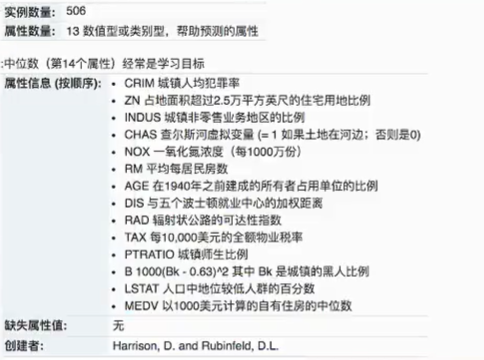
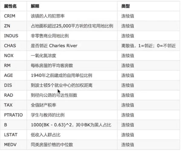
Technological process:
1) Get datasets
2) Partitioning datasets
3) Feature Engineering: No Dimension-Standardization
4) Estimator process: fit() ->model, coef_ intercept_
5) Model evaluation

2 Regression performance evaluation
Mean Square Error (MSE) Evaluation Mechanism

3 Code

from sklearn.datasets import load_boston
from sklearn.model_selection import train_test_split
from sklearn.preprocessing import StandardScaler
from sklearn.linear_model import LinearRegression, SGDRegressor
from sklearn.metrics import mean_squared_error


def linner1():
    """
    Optimizing Methods for Normal Equations
    :return:
    """
    # 1) Get data
    boston = load_boston()

    # 2) Partitioning datasets
    x_train, x_test, y_train, y_test = train_test_split(boston.data, boston.target, random_state=22)

    # 3) Standardization
    transfer = StandardScaler()
    x_train = transfer.fit_transform(x_train)
    x_test = transfer.transform(x_test)

    # 4) Estimator
    estimator = LinearRegression()
    estimator.fit(x_train, y_train)

    # 5) Derive the model
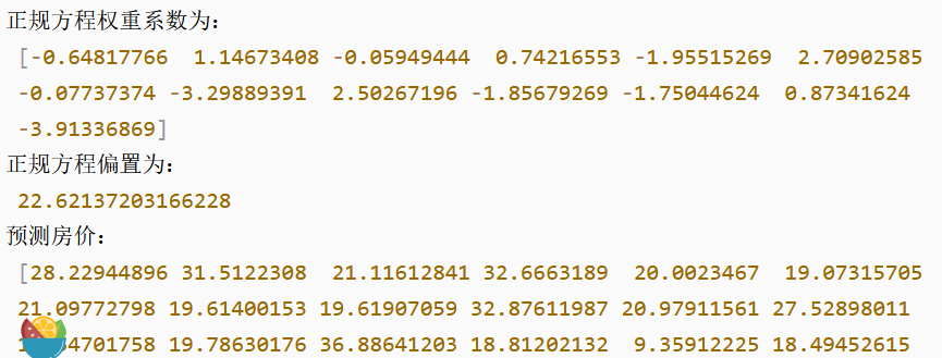
    print("The normal equation weight factor is:\n", estimator.coef_)
    print("The normal equation offset is:\n", estimator.intercept_)

    # 6) Model evaluation
    y_predict = estimator.predict(x_test)
    print("Forecast house prices:\n", y_predict)
    error = mean_squared_error(y_test, y_predict)
    print("Normal Equation-The average error is:\n", error)

    return None


def linner2():
    """
    Optimizing method for gradient descent
    :return:
    """
    # 1) Get data
    boston = load_boston()
    print("Number of features:\n", boston.data.shape)  # Several features correspond to several weight coefficients

    # 2) Partitioning datasets
    x_train, x_test, y_train, y_test = train_test_split(boston.data, boston.target, random_state=22)

    # 3) Standardization
    transfer = StandardScaler()
    x_train = transfer.fit_transform(x_train)
    x_test = transfer.transform(x_test)

    # 4) Estimator
    estimator = SGDRegressor(learning_rate="constant", eta0=0.001, max_iter=10000)
    estimator.fit(x_train, y_train)

    # 5) Derive the model
    print("The gradient descent weight factor is:\n", estimator.coef_)
    print("The gradient descent offset is:\n", estimator.intercept_)

    # 6) Model evaluation
    y_predict = estimator.predict(x_test)
    print("Forecast house prices:\n", y_predict)
    error = mean_squared_error(y_test, y_predict)
    print("gradient descent-The average error is:\n", error)

    return None


if __name__ == '__main__':
    linner1()
    linner2()

4. Case: Cancer Classification Prediction - Benign/Malignant Breast Cancer Prediction

Process analysis:
1) Get data: add names when reading
2) Data processing: processing missing values
3) Data Set Partition
4) Feature Engineering: Non-Dimensional Processing - Standardization
5) Logistic Regression Estimator
6) Model evaluation

Specific code

import pandas as pd
import numpy as np

# 1. Read Data
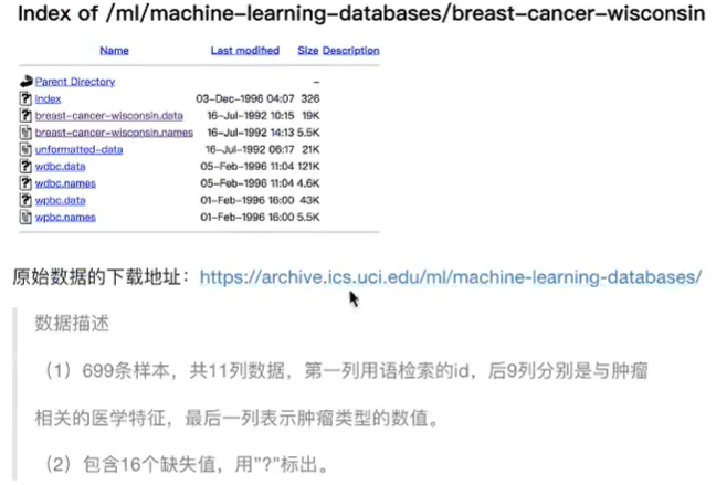
path = "https://archive.ics.uci.edu/ml/machine-learning-databases/breast-cancer-wisconsin/breast-cancer-wisconsin.data"
column_name = ['Sample code number', 'Clump Thickness', 'Uniformity of Cell Size', 'Uniformity of Cell Shape',
                   'Marginal Adhesion', 'Single Epithelial Cell Size', 'Bare Nuclei', 'Bland Chromatin',
                   'Normal Nucleoli', 'Mitoses', 'Class']

data = pd.read_csv(path, names=column_name)  #699 rows × 11 columns

# 2. Treatment of missing values
# 1) Replace - "np.nan
data = data.replace(to_replace="?", value=np.nan)
# 2) Delete missing samples
data.dropna(inplace=True)  #683 rows × 11 columns

# 3. Partitioning datasets
from sklearn.model_selection import train_test_split

# Screening Eigenvalues and Target Values
x = data.iloc[:, 1:-1]
y = data["Class"]

x_train, x_test, y_train, y_test = train_test_split(x, y)

# 4. Standardization
from sklearn.preprocessing import StandardScaler

transfer = StandardScaler()
x_train = transfer.fit_transform(x_train)
x_test = transfer.transform(x_test)

from sklearn.linear_model import LogisticRegression

# 5. Estimator process
estimator = LogisticRegression()
estimator.fit(x_train, y_train)

# Model parameters for logistic regression: regression coefficients and biases
estimator.coef_   # weight

estimator.intercept_  # bias

# 6. Model Evaluation
# Method 1: Direct comparison of true and predicted values
y_predict = estimator.predict(x_test)
print("y_predict:\n", y_predict)
print("Direct comparison of true and predicted values:\n", y_test == y_predict)

# Method 2: Calculate the accuracy
score = estimator.score(x_test, y_test)
print("Accuracy:\n", score)

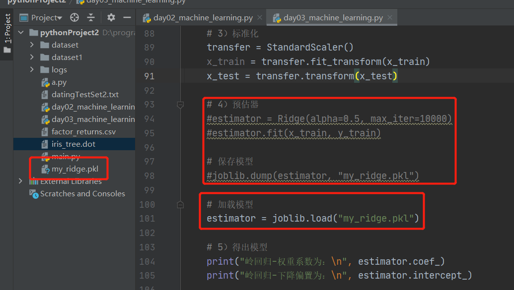
7. Model preservation and loading

import joblib

Preservation: joblib.dump(rf, 'test.pkl')
Load: estimator = joblib.load('test.pkl')

Case:

1. Save the model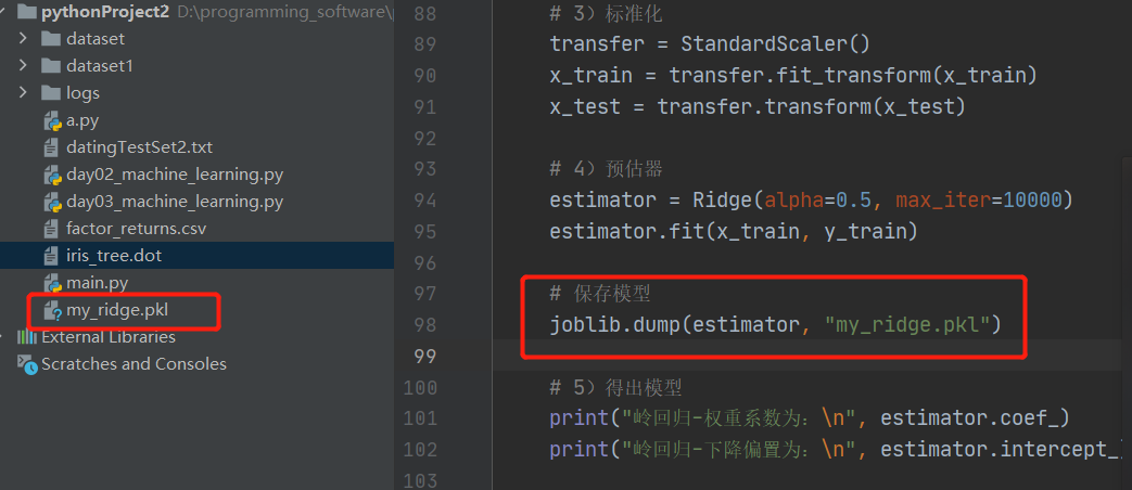

2. Loading models