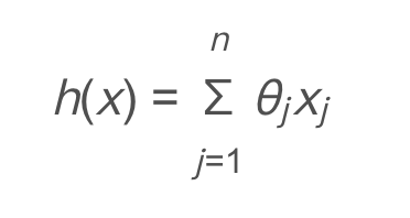
Multiple Features
Multiple linear regression, which includes multiple variables, such as house age, area, number of rooms, etc., is marked as follows:
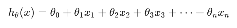
Suppose the function becomes:
It can be understood as:
θ 0 means base price
θ 1 is the price per square meter, and X1 is the number of square meters
θ 2 is the price of each floor and X2 is the number of floors
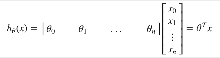
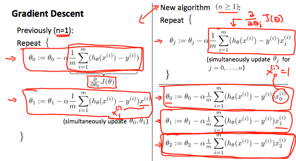
Suppose the function is abbreviated as:
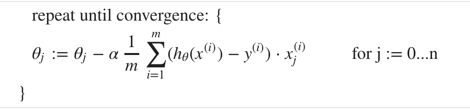
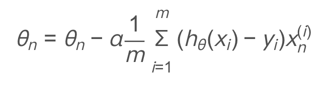
The gradient drop becomes:
The figure on the left shows the gradient decline in the previous univariate, and the figure on the right shows the gradient decline in multivariable. The comparison between the two is as follows:
Eigenvalue preprocessing
When the magnitude difference of several features is too large, the left figure will appear, and the convergence path is complex and slow;
It is better to scale the features close to [- 1,1], so that they can converge like the right figure to form round contours, accelerate convergence and reduce the number of iterations.
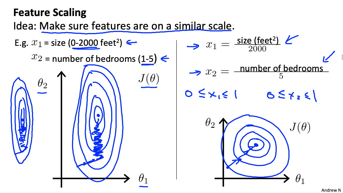
The following two techniques can be used.
Scaling feature
Divide the eigenvalue by Xmax - Xmin to get the new eigenvalue within 1.
mean normalization
Replace xi with xi - ui to bring the mean close to 0.
The two technologies are applied at the same time, that is, the following formula is adopted:
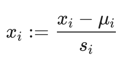
ui = mean(x)
si = xmax - xmin
Learning rate—— α
debug gradient learning
In order to ensure the normal operation of gradient descent, the image of iteration number cost function can be observed:
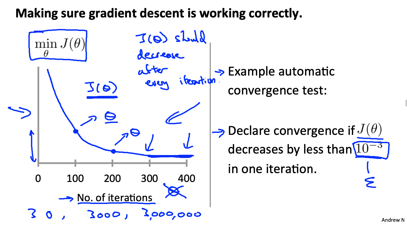
When J( θ) When the reduction is less than 10-3, it can be regarded as convergence.
Learning rate α Selection of
If α If it is too large, there may be two pictures on the left. Either J continues to grow or fluctuates up and down.
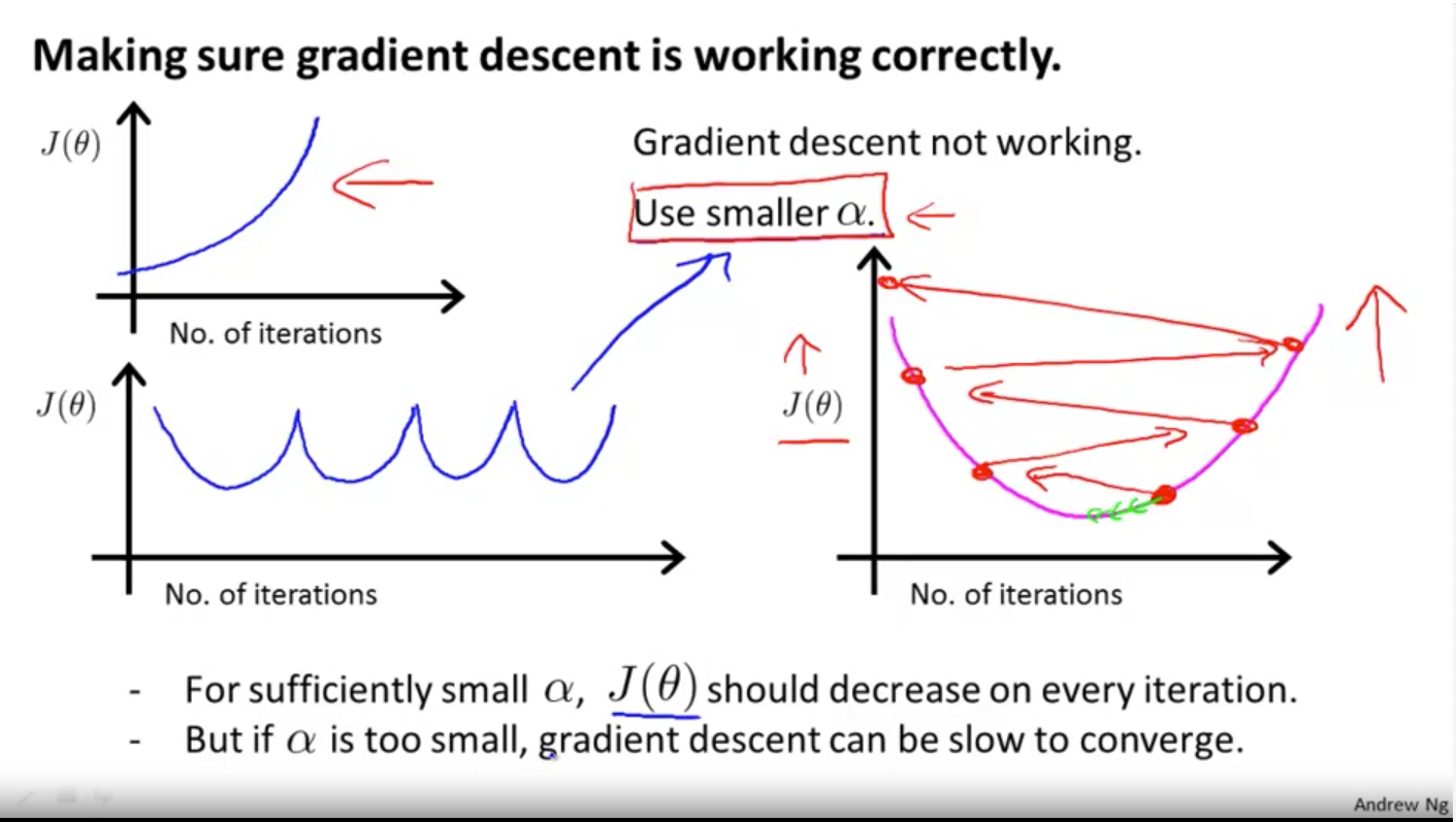
But if α Too small will cause too slow convergence. So try the following sequence:
α = 0.001,0.003,0.01, 0.03, 0.1, 0.3,1 ...
Draw the function diagram of J and iter above and observe the effect.
polynomial regression
Observe the relationship between area and price, and assume that the function is not necessarily linear, but also polynomial:
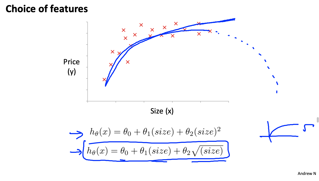
If the above polynomial function is selected, it is unreasonable to assume that the function will decrease when x continues to increase.
At this time, you can choose the square root function (or cubic function) in the blue box below.
Note that feature scaling is important at this time. The magnitude of X, X2, X3 can vary enormously.
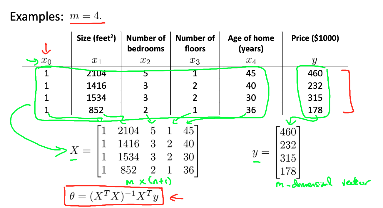
Normal Equation
Different from the gradient descent method, the normal equation can be solved directly by algebraic method θ Value.
That is, let each partial derivative be 0 and solve it θ Value:

For example, in the following example, after constructing X and Y, it can be calculated directly with the formula in the red box below θ Value of (why not delve into it first):
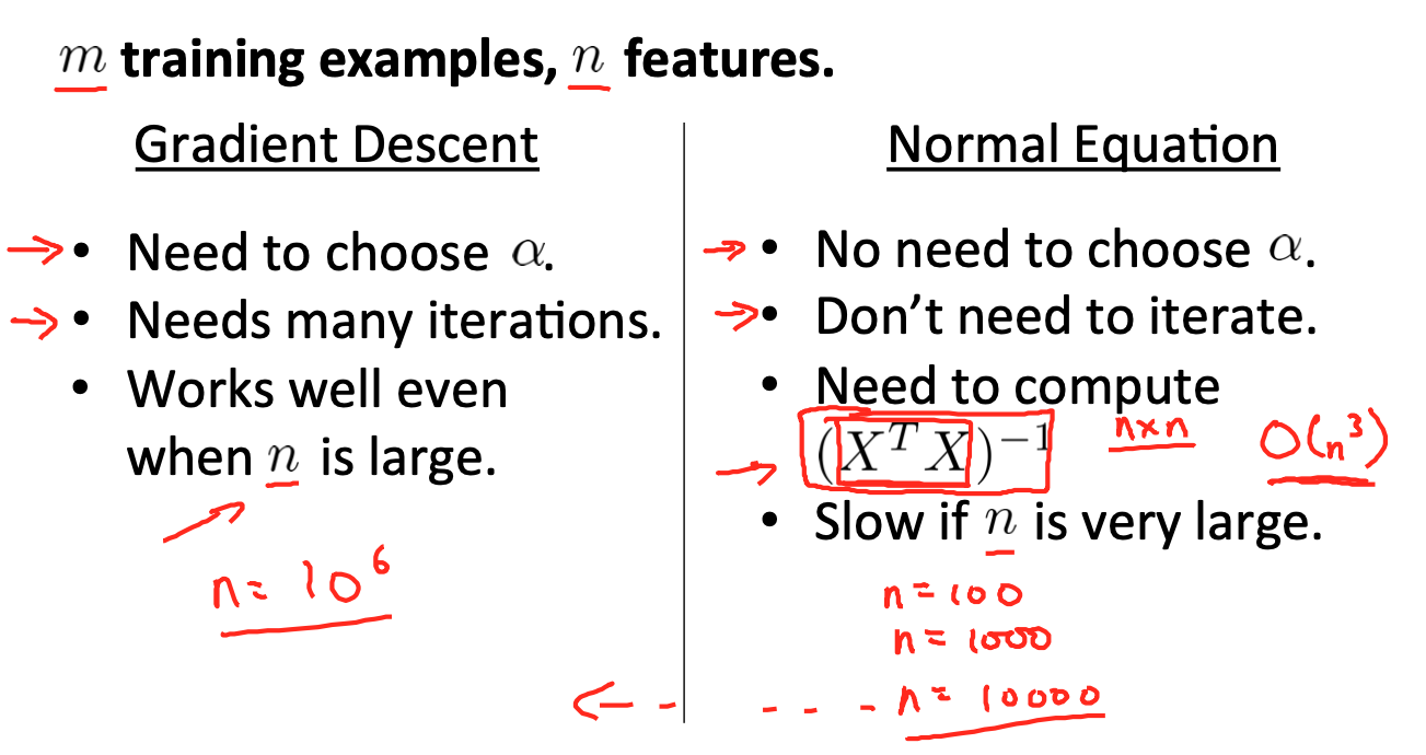
Contrast gradient descent method.
Gradient descent:
- Need to choose α
- Multiple iterations are required
- When n is very large, the effect is good, and the complexity is O(kn2)
Normal equation:
- No selection required α
- Multiple iterations are not required
- When n is large, XT X is an n * n matrix, and the transpose complexity of calculating n * n matrix is O(n3)
- Unable to solve problems such as logistic regression and classification
When n < 1000 (within 1000 characteristics), the normal equation will be used preferentially.
The case of XTX irreversibility in normal equation
- There are redundant features. For example, if x1 and x2 are linearly related, then XTX is irreversible.
- If there are too many features, such as m < = n, and the number of samples is less than the number of features, some features need to be deleted or regularized
Common operations of Matlab / Octave
reference resources: https://codeantenna.com/a/mVcQGKR7LB#1_3
Basic operation
Calculated value
>> 5 + 6
ans = 11
>> 3 * 4
ans = 12
>> 1/3
ans = 0.3333
>> 2^6
ans = 64
Calculate logical value
>> 1 == 2
ans = 0
>> 1 ~= 2
ans = 1
>> 1 && 0
ans = 0
>> 1 || 0
ans = 1
variable
>> a = 6
a = 6
>> a = 6;  %Adding a semicolon makes the variable not printout
>>
Print variables
>> a = pi;
>> a
a = 3.1416
>> disp(a)       %Output only a Value of
    3.1416
>> disp(sprintf("2 decimals : %0.2f",a))  %Print string (with c Language format)
2 decimals : 3.14
>>
Building matrices and vectors
>> A = [1 2;3 4;5 6]  %Semicolons represent line breaks in a matrix
A =
     1     2
     3     4
     5     6
>> v = [1 2 3]     %Represents a row vector (1)*3 (matrix of)
v =
     1     2     3
>> v = [1;2;3]     %Represents the column vector (3)*1 (matrix of)
v =
     1
     2
     3
>> v = 1:0.1:2   %Indicates from 1~2 Every 0.1 Take the number and get a row vector
v =
  1 To 8 columns
    1.0000    1.1000    1.2000    1.3000    1.4000    1.5000    1.6000    1.7000
  9 To 11 trains
    1.8000    1.9000    2.0000
>> v = 1:6       %Of course, the interval can also be omitted
v =
     1     2     3     4     5     6
Establishing matrix by special method
>> ones(2,3) %Build 2*3 Matrix with all elements of 1
ans =
1 1 1
1 1 1
>> 2*ones(2,3) %Use 2*Matrix, all elements are 2
ans =
2 2 2
2 2 2
>> zeros(2,2) %Generate zero matrix
ans =
0 0
0 0
>> rand(1,3) %Build 0~1 Random matrix of
ans =
0.8147 0.9058 0.1270
>> randn(1,3) %Generate a Gaussian distribution matrix (normal distribution) with a mean of 0 and a standard deviation of 1
ans =
0.8622 0.3188 -1.3077
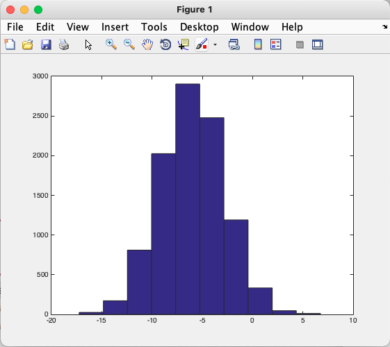
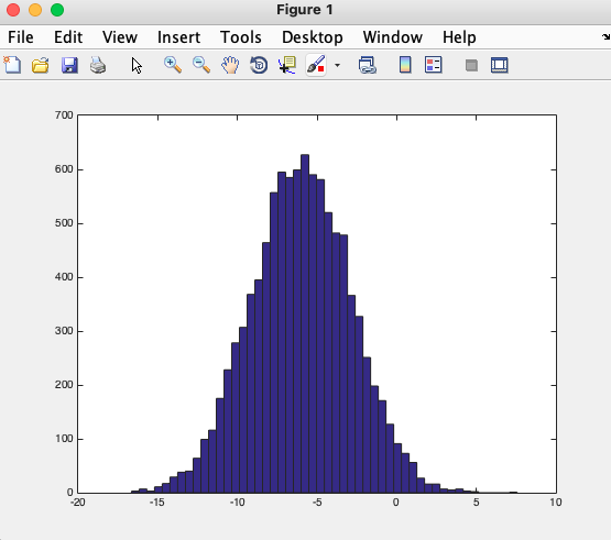
>> >> w = -6 + sqrt(10)*(randn(1,10000)); % The generated mean is-6,Matrix of 10000 data with variance of 10
>> hist(w) %Draw the matrix in the form of histogram
>> hist(w,50) %Histogram display with 50 vertical bars
>> eye(4)   %Generate identity matrix
ans =
     1     0     0     0
     0     1     0     0
     0     0     1     0
     0     0     0     1
>> eye(3)
ans =
     1     0     0
     0     1     0
     0     0     1
mobile data
Size of matrix
>> A = [1 2;3 4;5 6]
A =
     1     2
     3     4
     5     6
>> size(A)      %size()You can view the size of the matrix
ans =
     3     2
>> s = size(A)
s =
     3     2
>> size(s)        %size()What it returns is a matrix
ans =
     1     2
>> size(A,1)     %Will return A Size of the first dimension of the matrix (number of rows)
ans =
     3
>> size(A,2)     %Will return A Size of the second dimension of the matrix (number of columns)
ans =
     2
>> v = [1 2 3 4]
v =
     1     2     3     4
>> length(v)      %Returns the length of the row vector
ans =
     4
>> length(A)   %Returns the larger dimension length 3
ans =
     3
load file
>> load('ex1data1.txt')   %use load The data in the file can be read out directly
>> who           %Displays the variables for the current workspace

Your variables are:

A         ans       ex1data1  s         v

>> size(ex1data1)       %Just read the matrix and check the length
ans =
    97     2
>> whos   %View the details of the current workspace variable
  Name           Size            Bytes  Class     Attributes

  A              3x2                48  double
  ans            1x1                 8  double
  ex1data1      97x2              1552  double
  s              1x2                16  double
  v              1x4                32  double
>> clear(v)   %Delete variables, and delete all variables without specifying
>> v = ex1data1(1:10)  %Take the first 10 elements
v =
  1 To 8 columns
    6.1101    5.5277    8.5186    7.0032    5.8598    8.3829    7.4764    8.5781
  9 To 10 trains
    6.4862    5.0546
>> save v.mat v    %take v The data in the matrix is saved to a file v.mat Zhongqu
The above is stored in binary format and compressed. If you want to make it easy to read, you can use the following parameters:
>> save v.txt v -ascii
Operation matrix data
>> A
A =
     1     2
     3     4
     5     6
>> A(3,2)  %take A Elements in the third row and second column of a matrix
ans =
     6
>> A(2,:)   %take A All elements in the second row of the matrix
ans =
     3     4
>> A(:,2)   %Take all the elements in the second column
ans =
     2
     4
     6
>> A([1 3],:)    %take A All elements of the first and third rows of the matrix
ans =
     1     2
     5     6
>> A(:,2) = [10 15 20]  %After taking out the element, you can actually assign a value to it
A =
     1    10
     3    15
     5    20
>> A = [A,[100;150;200]] %stay A Add a column after the matrix
A =
     1    10   100
     3    15   150
     5    20   200
>> A(:)    %hold A All elements of the matrix are placed in a column vector
ans =
     1
     3
     5
    10
    15
    20
   100
   150
   200
>> A = [1 2;3 4;5 6];
>> B = [11 12;13 14;15 16];
>> C = [A,B]     %Splice the two matrices together
C =
     1     2    11    12
     3     4    13    14
     5     6    15    16
>> C = [A;B]      %Semicolons indicate line breaks, B Matrix on A Below the matrix
C =
     1     2
     3     4
     5     6
    11    12
    13    14
    15    16
Calculation data
Inter matrix operation
>> A = [1 2;3 4;5 6];
>> B = [11 12;13 14;15 16];
>> C = [1 1;2 2]
C =
     1     1
     2     2
>> A * C     %A And C Matrix multiplication
ans =
     5     5
    11    11
    17    17
>> A .* B      %'.*'Multiplication of corresponding elements in representative matrix
ans =
    11    24
    39    56
    75    96
>> A .^ 2     %'.'Represents the power of all elements in the matrix
ans =
     1     4
     9    16
    25    36
>> v = [1 2 3]
>> v = 1 ./ v    %take v Reciprocal of matrix
v =
    1.0000    0.5000    0.3333
>> log(v)     %yes v take log operation
ans =
         0   -0.6931   -1.0986
>> exp(v)      %yes v take e^v Power operation
ans =
    2.7183    1.6487    1.3956
>> abs([-1;-2;3])  %Operation of taking absolute value of matrix
ans =
     1
     2
     3
>> -v          %Take the opposite number of the matrix
ans =
   -1.0000   -0.5000   -0.3333
>> v = [1;2;3];
>> v = v + ones(length(v),1) %take v All elements in+1,First construct a sum v Matrices with the same dimension (all elements are 1), and then add them
v =
     2
     3
     4
>> v = v +1     %Actually use+No. 1 can be realized
v =
     3
     4
     5
>> A'      %An apostrophe is the transpose of a matrix
ans =
     1     3     5
     2     4     6
function
>> a = [-0.2 9.8 4.5 8 2.0]
a =
   -0.2000    9.8000    4.5000    8.0000    2.0000
>> val = max(a)   %Find the maximum value of the matrix
val =
    9.8000
>> [val index] = max(a)    %Find the maximum value of the matrix and return its subscript index
val =
    9.8000
index =
     2
>> a < 3     %take a Compare all elements in and 3 to return results
ans =
  1×5 logical array
   1   0   0   0   1
>> find(a<3)   %Returns the element that meets the condition a Index in
ans =
     1     5
>>A = magic(3)  %Magic square matrix, the sum of diagonal elements in each row and column is equal
 A =
     8     1     6
     3     5     7
     4     9     2
>> [r,c] = find(A>=7)  %seek A Element indexes, rows and columns greater than or equal to 7 in
r =
     1
     3
     2
c =
     1
     2
     3
>> sum(a)    %Sum the elements in the matrix
ans =
   24.1000
>> prod(a)    %Multiply the elements in the matrix
ans =
 -141.1200
>> floor(a)    %Round down
ans =
    -1     9     4     8     2
>> ceil(a)      %Round up
ans =
     0    10     5     8     2
>> A
A =
     8     1     6
     3     5     7
     4     9     2
>> max(A) %The default value is the maximum value of each column
ans =
     8     9     7
>> max(A,[],1)   %Take the maximum value of each column, and 1 represents the first dimension
ans =
     8     9     7
>> max(A,[],2)   %Take the maximum value of each row
ans =
     8
     7
     9
>> max(max(A))  %take A Maximum value of all elements of the matrix
ans =
     9
>> max(A(:))  %Or you can start with the matrix A Convert to column vector and take the maximum value in
ans =
     9
>> sum(A,1)  %seek A Sum of each column
ans =
    15    15    15
>> sum(A,2) %seek A Sum of each line
ans =
    15
    15
    15
>> A .* eye(3)   %Combine identity matrix with A Multiply the elements in to get the diagonal elements
ans =
     8     0     0
     0     5     0
     0     0     2
>> sum(sum(A .* eye(3)))  %Find the sum of diagonal elements
ans =
    15
>> pinv(A)    %Inverse matrix
ans =
    0.1472   -0.1444    0.0639
   -0.0611    0.0222    0.1056
   -0.0194    0.1889   -0.1028
>> temp = pinv(A);
>> A*temp     %It is found that this is the identity matrix
ans =
    1.0000   -0.0000    0.0000
    0.0000    1.0000   -0.0000
   -0.0000    0.0000    1.0000
Draw data
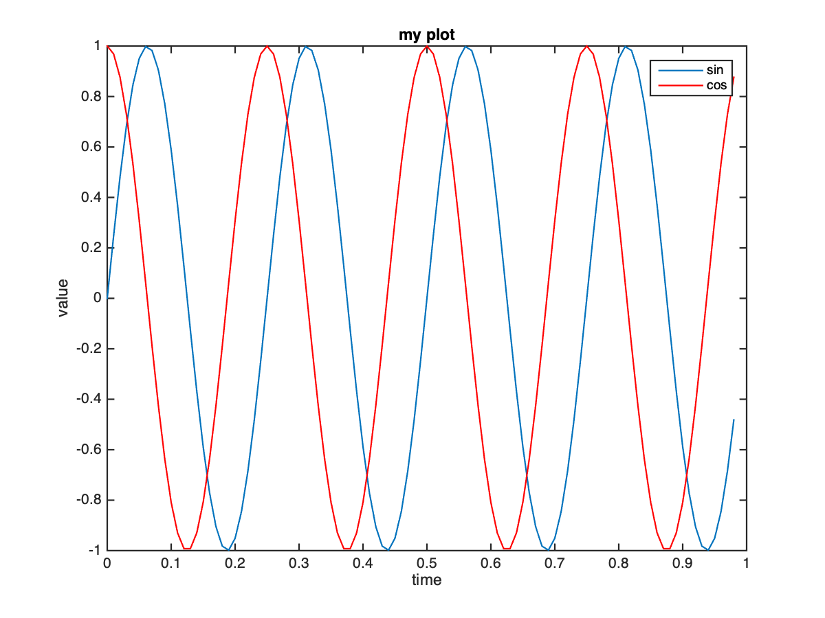
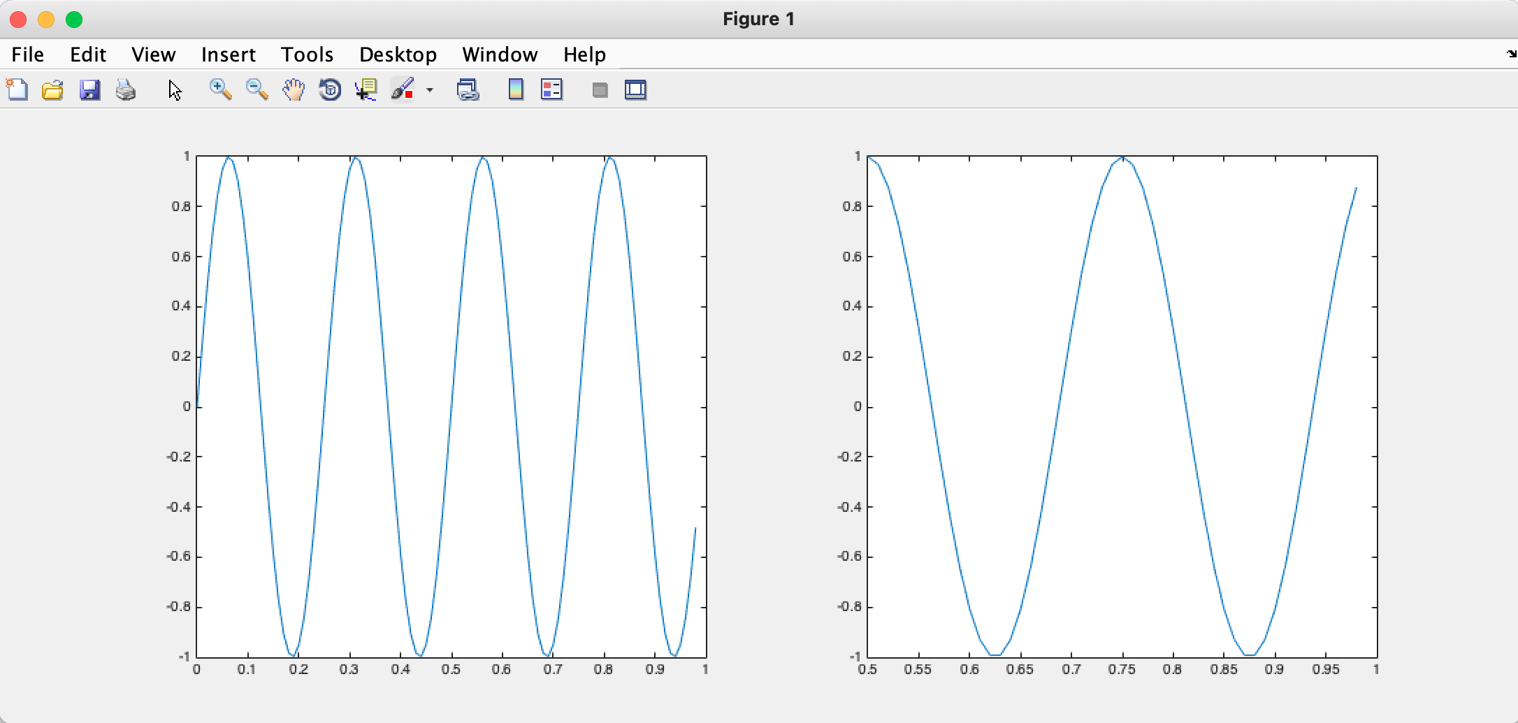
>> t = [0:0.01:0.98];
>> y1 = sin(2*pi*4*t);
>> plot(t,y1);   %use plot You can draw the corresponding sin Function image
>> y2 = cos(2*pi*4*t);
>> hold on;     %Draw images on the same interface
>> plot(t,y2,'r');   %Draw cos Function image, using red
>> xlabel('time');    %set up x Axis coordinates
>> ylabel('value');   %set up y Axis coordinates
>> legend('sin','cos');  %Set identity
>> title('my plot');   %Set title
>> print -dpng 'myplot.PNG';  %Save image as PNG format
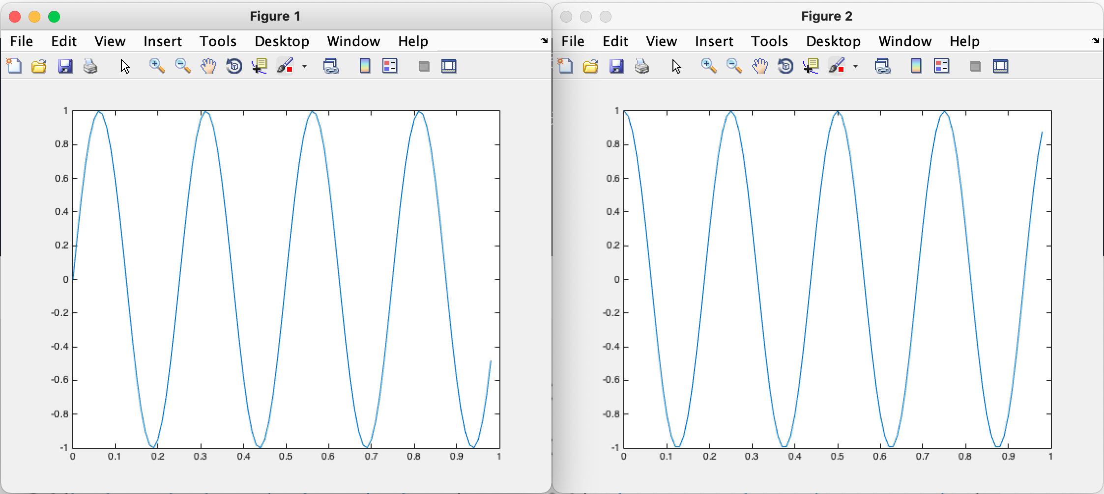
>> figure(1); plot(t,y1);  %Label the images so that each image has an interface
>> figure(2); plot(t,y2);
>> subplot(1,2,1);    %Divide the interface into 1*2 Use the first area
>> plot(t,y1);     %First area painting y1 Image of
>> subplot(1,2,2);    %Use the second area
>> plot(t,y2);      %The second area painting y2 Image of
>> axis([0.5 1 -1 1]);   %Set the abscissa and ordinate range of the image
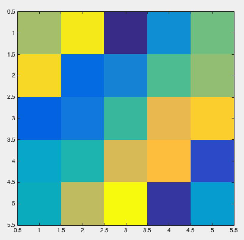
>> A = magic(5)  %5*5 Magic square matrix of
A =
    17    24     1     8    15
    23     5     7    14    16
     4     6    13    20    22
    10    12    19    21     3
    11    18    25     2     9
>> imagesc(A);   %The matrix can also be visualized
Process control
>> v = zeros(10,1)
>> for i = 1:10,  %i = 1:10,Then put v(i)The value of becomes 2 i Power
     v(i) = 2^i;
   end            %Pay attention to adding at the end end
>> v
v =
           2
           4
           8
          16
          32
          64
         128
         256
         512
        1024
>> i = 1;
>> while true,    %while loop
     v(i) = 999;  %set up v(i)The value of is 999
     i = i + 1;
     if i == 6,  %When i=6 Jump out of loop when
        break;
     end
  end
>> v
v =
         999
         999
         999
         999
         999
          64
         128
         256
         512
        1024
function
Store the following code as squarethisnumber m:
function y = squareThisNumber(x) %y Is the return value, x Parameters passed in for
    y = x^2
end
Execute the following statement in this directory to call this function:
>> squareThisNumber(5);
y =
    25
Functions with multiple return values:
function [a,b] = squareTwoNumber(x)
    a = x^2
    b = x^3
end
>> squareTwoNumber(5) %y Is the return value, x Parameters passed in for

a =

    25


b =

   125


ans =

    25
The cost function is defined as follows:
function J = costFunctionJ(X,y,theta)
    m = size(X,1);       %Number of data sets
    predictions = X*theta;    %Result matrix of hypothetical function prediction
    sqrErrors = (predictions - y) .^ 2;   %Error from actual value
    J = 1/(2*m) * sum(sqrErrors);     %Calculation cost function
end
Call function:
>> X = [1 1;1 2;1 3];
>> Y = [1;2;3];
>> X
X =
     1     1
     1     2
     1     3
>> Y
Y =
     1
     2
     3
>> theta = [0;1]
theta =
     0
     1
>> costFunctionJ(X,Y,theta)  %theta0=0,theta0=1 Just fit, so the cost function is 0
ans =
     0
>> theta = [0;0]
theta =
     0
     0
>> costFunctionJ(X,Y,theta)
ans =
    2.3333
Vectorization
Vectorized code will be simpler and clearer.
Hypothetical function
The hypothetical function formula on the left can be calculated by vectorization on the right:
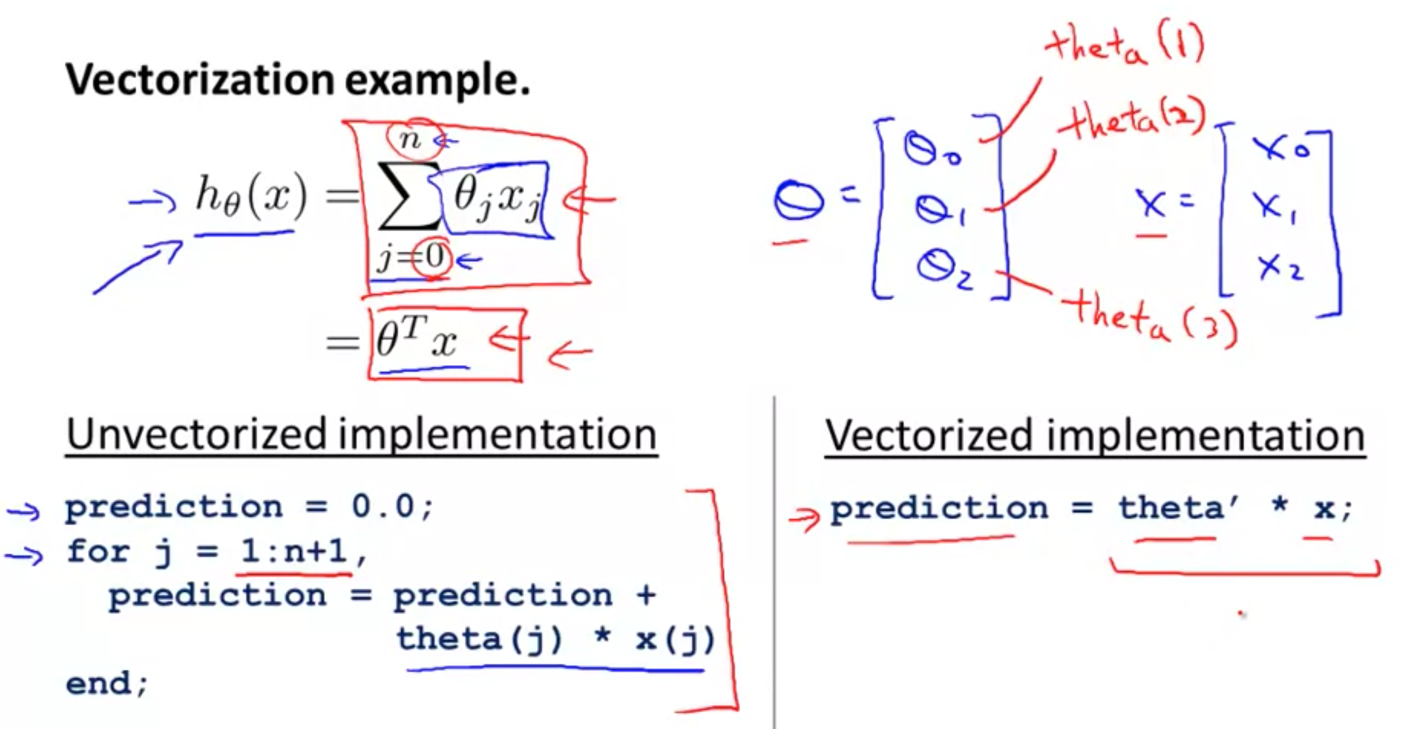
Hypothetical function:
matlab function:
function pre = prediction(X,theta)
   pre = theta' * X;  % ' Transpose of representative matrix
end
gradient descent

Gradient descent update formula:
matlab code:
function Theta = UpdateTheta(X,Y,theta,alpha)
    m = size(X,1);
    Error = X * theta - Y;
    delta = alpha/m * (X' * Error);
    Theta = theta - delta;
end
task
warmUpExercise.m
function A = warmUpExercise()
%WARMUPEXERCISE Example function in octave
%   A = WARMUPEXERCISE() is an example function that returns the 5x5 identity matrix
% ============= YOUR CODE HERE ==============
% Instructions: Return the 5x5 identity matrix
%               In octave, we return values by defining which variables
%               represent the return values (at the top of the file)
%               and then set them accordingly.

A = eye(5);
% ===========================================
end
plotData.m
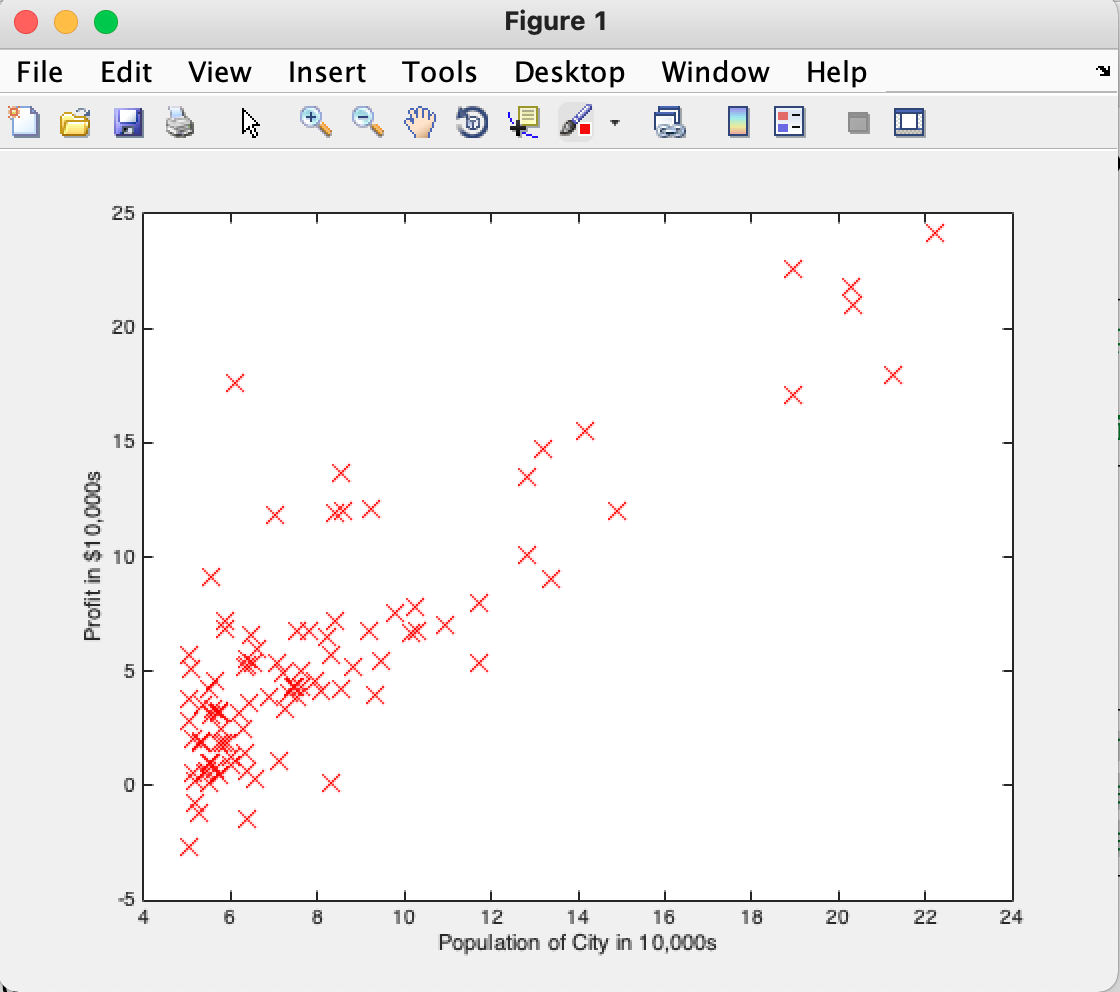
function plotData(x, y)
%PLOTDATA Plots the data points x and y into a new figure
%   PLOTDATA(x,y) plots the data points and gives the figure axes labels of
%   population and profit.

figure; % open a new figure window

% ====================== YOUR CODE HERE ======================
% Instructions: Plot the training data into a figure using the
%               "figure" and "plot" commands. Set the axes labels using
%               the "xlabel" and "ylabel" commands. Assume the
%               population and revenue data have been passed in
%               as the x and y arguments of this function.
%
% Hint: You can use the 'rx' option with plot to have the markers
%       appear as red crosses. Furthermore, you can make the
%       markers larger by using plot(..., 'rx', 'MarkerSize', 10);

plot(x, y, 'rx', 'MarkerSize', 10); % Plot the data
ylabel('Profit in $10,000s'); % Set the y−axis label
xlabel('Population of City in 10,000s'); % Set the x−axis label

% ============================================================

end
computeCost.m
function J = computeCost(X, y, theta)
%COMPUTECOST Compute cost for linear regression
%   J = COMPUTECOST(X, y, theta) computes the cost of using theta as the
%   parameter for linear regression to fit the data points in X and y

% Initialize some useful values
m = length(y); % number of training examples

% You need to return the following variables correctly
% J = 0;

% ====================== YOUR CODE HERE ======================
% Instructions: Compute the cost of a particular choice of theta
%               You should set J to the cost.

h = X * theta;
sqrErrors = (h - y) .^ 2;
J = 1 / (2 * m) * sum(sqrErrors);


% =========================================================================

end
gradientDescent.m
function [theta, J_history] = gradientDescent(X, y, theta, alpha, num_iters)
%GRADIENTDESCENT Performs gradient descent to learn theta
%   theta = GRADIENTDESCENT(X, y, theta, alpha, num_iters) updates theta by
%   taking num_iters gradient steps with learning rate alpha

% Initialize some useful values
m = length(y); % number of training examples
J_history = zeros(num_iters, 1);

for iter = 1:num_iters

    % ====================== YOUR CODE HERE ======================
    % Instructions: Perform a single gradient step on the parameter vector
    %               theta.
    %
    % Hint: While debugging, it can be useful to print out the values
    %       of the cost function (computeCost) and gradient here.
    %
    theta = theta - alpha / m * (X' * (X * theta - y))


    % ============================================================

    % Save the cost J in every iteration
    J_history(iter) = computeCost(X, y, theta);

end

end
Gradient descent formula:
theta = theta - alpha / m * (X' * (X * theta - y))
Where x * ta - M is the matrix,
X 'is (n+1) * m matrix,
(x '* (x * theta - y)) is the (n+1) * 1 matrix,
alpha / m is a scalar,
As a result, theta is still a (n+1) * 1 matrix.
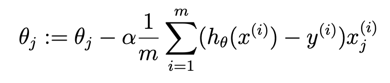
The last xj(i), when j=0, is x0(i), which uses column 0 of X.
Update each θ, Only the value of one dimension corresponding to X is used.
Therefore, the matrix updated each time is alpha / m * (x '* (x * theta - y)), X' transposes x, and each multiplication uses a column of values.