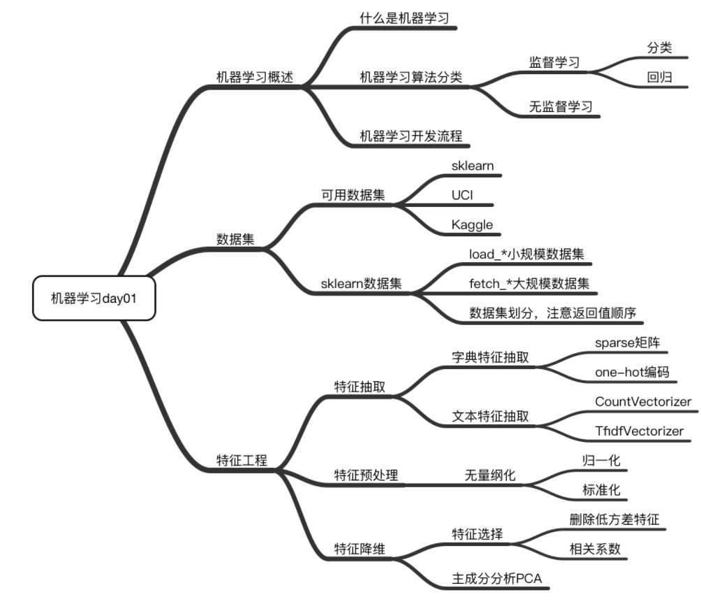
I Machine learning overview
Watch the introduction video of dark horse programmer's machine learning at station B and write this note to consolidate knowledge.
Video link of station B
Relevant information can be found in the comment area of the video.
1.1 definition:
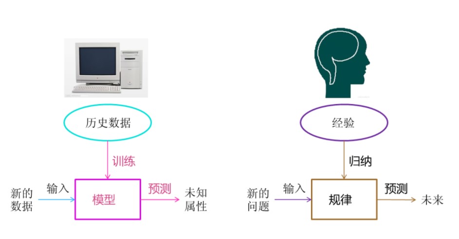
Machine learning is to automatically analyze and obtain the model from the data, and use the model to predict the unknown data.
1.2 composition of machine learning data set
Structures: eigenvalues +  target value

For example, the data structure shown in the figure below

For each row of data, we can call it**sample**
Some datasets have no target values
1.3. Classification of machine learning algorithms
It is mainly divided into two categories: supervised learning and unsupervised learning
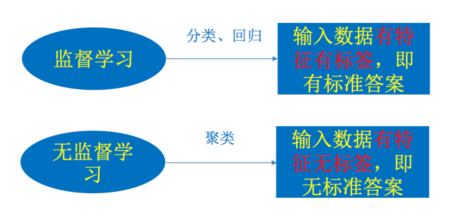
Supervised learning (prediction)
Definition: input data is composed of input characteristic value and target value. The output of the function can be
 A continuous value(Called regression), or the output is a finite number of discrete values (called classification).
Classification algorithm:
k-Nearest neighbor algorithm, Bayesian classification, decision tree and random forest, logistic regression, neural network
Regression algorithm
Linear regression, ridge regression
Unsupervised learning
Definition: input data is composed of input characteristic values.

clustering k-means
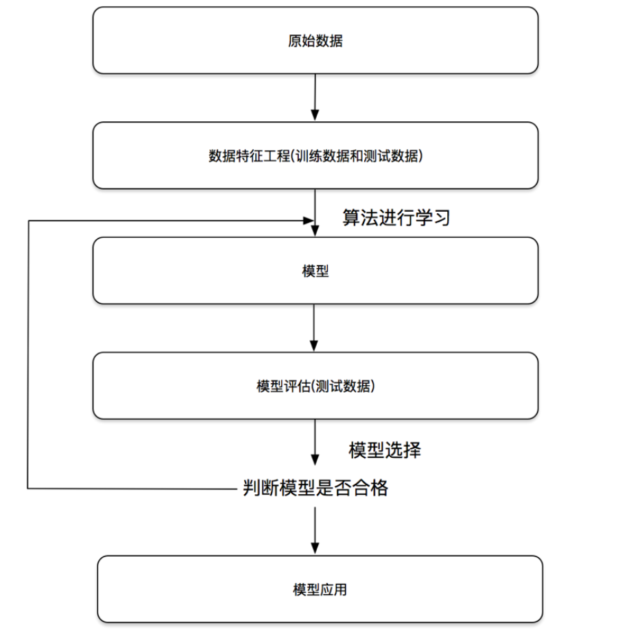
1.4 machine learning development process:
II Characteristic Engineering
Use sklearn library to operate feature engineering
2.1 obtaining data sets
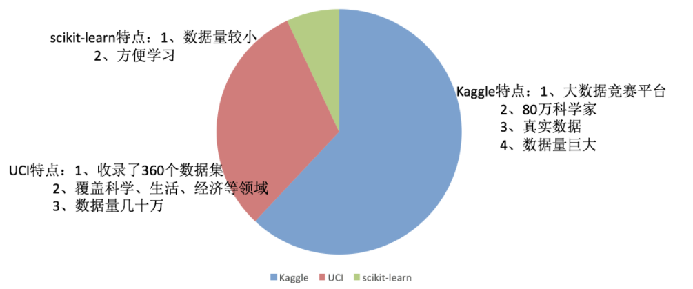
The following are the websites of three data sets:
Kaggle website: https://www.kaggle.com/datasets
UCI dataset website: http://archive.ics.uci.edu/ml/
Scikit learn website:
http://scikit-learn.org/stable/datasets/index.html#datasets
Or get data from the company
2.2 introduction to sklearn tool library
2.2.1 installation
Scikit-learn==0.19.1
Note: numpy, scipy and other libraries are required before downloading
Using sklearn to get started with machine learning generally uses two classic data sets, iris data set and Boston house price prediction data set.
Iris dataset:

Boston house price forecast dataset:

2.2.2 API for reading data sets
sklearn.datasets
 Load get popular dataset
datasets.load_*()
Obtain a small data set, and the data is contained in datasets in
datasets.fetch_*(data_home=None)
To obtain large-scale data sets, you need to download them from the network. The first parameter of the function is
data_home Represents the directory where the dataset is downloaded,Default is ~/scikit_learn_data/
Small data set:
sklearn.datasets.load_iris()
#Load and return iris dataset
sklearn.datasets.load_boston()
#Load and return Boston house price dataset
Big data set:
sklearn.datasets.fetch_20newsgroups(data_home=None,subset='train')
#subset: 'train' or 'test', 'all', optional. Select the dataset to load.
#"Training" of training set, "testing" of test set, and "all" of both
2.2.3 use of dataset API (take iris as an example)

Return value:
load and fetch Data product type returned datasets.base.Bunch(Dictionary format)
· data: Feature data array, yes[n_samples * n_features] Binary array of
· target: Tag array, yes n_sample One dimensional array of numpy.ndarrray array
· DESRCR: data description
· feature_name: Special certificate name, news data, handwritten digits and regression data set are not available
· target_names: Tag name
from sklearn.datasets import load_iris
# Get iris dataset
iris = load_iris()
print("Return value of iris dataset:\n", iris)
# The return value is a Bench inherited from the dictionary
print("Eigenvalues of iris:\n", iris["data"])
print("Target value of iris:\n", iris.target)
print("Iris characteristic Name:\n", iris.feature_names)
print("Name of iris target value:\n", iris.target_names)
print("Description of iris:\n", iris.DESCR)
2.2.4 data set division:
The general data set of machine learning is divided into two parts:
·Training data: used for training and building models
·Test data: used in model verification to evaluate whether the model is effective
 Division proportion:
·Training set: 70% 80% 75%
·Test set: 30% 20% 30%
Divided API:
sklearn.model_selection.train_test_split(arrays,*options)
x: Eigenvalues of data sets
y: Label value of the dataset
test_size: The size of the test set is generally float
random_state:Random number seeds, different seeds will cause different random sampling results. If the seeds are the same, the result page is the same.
return: Test set feature, training set feature value, training label, test label (random by default)
from sklearn.datasets import load_iris
from sklearn.model_selection import train_test_split


def datasets_demo():
    """
    Demonstration of iris dataset
    :return: None
    """
    # 1. Get iris dataset
    iris = load_iris()
    print("Return value of iris dataset:\n", iris)
    # The return value is a Bench inherited from the dictionary
    print("Eigenvalues of iris:\n", iris["data"])
    print("Target value of iris:\n", iris.target)
    print("Iris characteristic Name:\n", iris.feature_names)
    print("Name of iris target value:\n", iris.target_names)
    print("Description of iris:\n", iris.DESCR)

    # 2. Segmentation of iris data set
    # Eigenvalue X of training set_ Eigenvalue X of train test set_ Target value y of test training set_ Target value y of train test set_ test
    x_train, x_test, y_train, y_test = train_test_split(iris.data, iris.target, random_state=22)
    print("x_train:\n", x_train.shape)
    # Random number seed
    x_train1, x_test1, y_train1, y_test1 = train_test_split(iris.data, iris.target, random_state=6)
    x_train2, x_test2, y_train2, y_test2 = train_test_split(iris.data, iris.target, random_state=6)
    print("If the random number seeds are inconsistent:\n", x_train == x_train1)
    print("If the random number seeds are consistent:\n", x_train1 == x_train2)

    return None
2.3 introduction to characteristic Engineering
Feature engineering uses professional background knowledge and skills to process data, yes·Feature can play a better role in machine learning algorithm.

pandas: a very convenient tool for data reading and basic processing format.
sklearn: provides a powerful interface for feature processing.
Contents included:
feature extraction
Feature preprocessing
Feature dimensionality reduction
2.4 feature extraction
2.4.1. Why feature extraction
The original data is often high-dimensional, which contains a lot of redundant information, or very sparse or large amount of calculation. It is feasible to train with the original data, but it is often inefficient to train directly. Therefore, feature extraction is often necessary.
Note: 1 Feature extraction is mainly to solve the following three problems.
(1) Redundant information caused by strong correlation in original data features. (2) The original data is very sparse. (3) The original data dimension is huge
2. Feature extraction is to make the computer better understand the data.
2.4.2 contents:
 Dictionary feature extraction (feature discretization)
 Text feature reading
 Image feature reading (deep learning)
2.4.3 dictionary feature extraction API
sklearn.feature_extraction.DictVectorizer(sparse=True,...)
	DictVectorizer.fit_transform(X) X:Return value of dictionary or iterator containing Dictionary: sparse matrix
	DictVectorizer.inverse_transform(X) X:array Array or sparse Matrix return value:Data format before conversion
	DictVectorizer.get_feature_names() Return category name
Note: if there are categories in the features, they are generally 0ne-hot coded
EX:
#1. Instantiate the class DicVectorize
#Call fit_transform method converts data (pay attention to the returned data type)
from sklearn.feature_extraction import DicVectorize

def dict_demo():
	data = [{'city': 'Beijing','temperature':100}, {'city': 'Shanghai','temperature':60}, {'city': 'Shenzhen','temperature':30}]
    # 1. Instantiate a converter class
    transfer = DictVectorizer(sparse=False) #Here is spark = false
    # 2. Call fit_transform
    data = transfer.fit_transform(data)
    print("Returned results:\n", data)
    # Print feature name
    print("Feature Name:\n", transfer.get_feature_names())

    return None
Return result:
(0, 1)    1.0
(0, 3)    100.0
(1, 0)    1.0
(1, 3)    60.0
(2, 2)    1.0
(2, 3)    30.0
 Feature Name:
['city=Shanghai', 'city=Beijing', 'city=Shenzhen', 'temperature']
If spark = true
Return result:
Returned results:
[[   0.    1.    0.  100.]
[   1.    0.    0.   60.]
[   0.    0.    1.   30.]]
Feature Name:
['city=Shanghai', 'city=Beijing', 'city=Shenzhen', 'temperature']
2.4.4 text data feature extraction API
sklearn.feature_extraction.text.CountVectorizer(stop_words=[])     Return word frequency matrix
	CountVectorizer.fit_transform(X) X:Return value of text or iteratable object containing text string: sparse matrix
	CountVectorizer.inverse_transform(X) X:array Array or sparse Matrix return value:Data grid before conversion
	CountVectorizer.get_feature_names() Return value:Word list
	sklearn.feature_extraction.text.TfidfVectorizer
EX:
#1. Instantiate the class CountVectorizer
#2. Call fit_ The transform method inputs the data and converts it (pay attention to the return format, and use toarray() to convert the sparse matrix into an array)
from sklearn.feature_extraction.text import CountVectorizer

def text_count_demo():
    """
    Feature extraction of text, countvetorizer
    :return: None
    """
    data = ["life is short,i like like python", "life is too long,i dislike python"]
    # 1. Instantiate a converter class
    # transfer = CountVectorizer(sparse=False)
    transfer = CountVectorizer()
    # 2. Call fit_transform
    data = transfer.fit_transform(data)
    print("Results of text feature extraction:\n", data.toarray())
    print("Return feature Name:\n", transfer.get_feature_names())

    return None
Return result:
Results of text feature extraction:
[[0 1 1 2 0 1 1 0]
[1 1 1 0 1 1 0 1]]
Return feature Name:
['dislike', 'is', 'life', 'like', 'long', 'python', 'short', 'too']
If the processed data is Chinese, you need to use the jieba library
jieba.cut()
Returns a generator of words
 Need to install jieba library
pip3 install jieba
Case:
Characterize the following text
Today is cruel, tomorrow is more cruel, and the day after tomorrow is beautiful,
But most of them will die tomorrow night, so don't give up today.

The light we see from distant galaxies was emitted millions of years ago,
So when we see the universe, we are looking at its past.

If you only know something in one way, you won't really know it.
The secret of understanding the true meaning of things depends on how to connect them with what we know.
analysis:
Prepare sentences using jieba.cut Progressive participle
 instantiation  CountVectorizer
 Turn the word segmentation result into a string as fit_transform Input value of
from sklearn.feature_extraction.text import CountVectorizer
import jieba

def cut_word(text):
    """
    Chinese word segmentation
    "I Love Beijing Tiananmen "-->"I love Beijing Tiananmen Square"
    :param text:
    :return: text
    """
    # Word segmentation of Chinese string by stuttering
    text = " ".join(list(jieba.cut(text)))

    return text

def text_chinese_count_demo2():
    """
    Feature extraction of Chinese
    :return: None
    """
    data = ["One kind or another, today is cruel, tomorrow is more cruel, and the day after tomorrow is beautiful, but most of them die tomorrow night, so everyone should not give up today.",
            "The light we see from distant galaxies was emitted millions of years ago, so when we see the universe, we are looking at its past.",
            "If you only know something in one way, you won't really know it. The secret of understanding the true meaning of things depends on how to connect them with what we know."]
    # Convert the original data into the form of good words
    text_list = []
    for sent in data:
        text_list.append(cut_word(sent))
    print(text_list)

    # 1. Instantiate a converter class
    # transfer = CountVectorizer(sparse=False)
    transfer = CountVectorizer()
    # 2. Call fit_transform
    data = transfer.fit_transform(text_list)
    print("Results of text feature extraction:\n", data.toarray())
    print("Return feature Name:\n", transfer.get_feature_names())

    return None
Return results
Building prefix dict from the default dictionary ...
Dumping model to file cache /var/folders/mz/tzf2l3sx4rgg6qpglfb035_r0000gn/T/jieba.cache
Loading model cost 1.032 seconds.
['One or another, today is cruel, tomorrow is more cruel, and the day after tomorrow is beautiful, but most of them die tomorrow night, so everyone 		Don't give up today.', 'The light we see from distant galaxies was emitted millions of years ago, so when we see the universe, we are looking at its past.', 'If you only know something in one way, you won't really know it. The secret of understanding the true meaning of things depends on how to connect them with what we know.']
Prefix dict has been built succesfully.
Results of text feature extraction:
 [[2 0 1 0 0 0 2 0 0 0 0 0 1 0 1 0 0 0 0 1 1 0 2 0 1 0 2 1 0 0 0 1 1 0 0 1 0]
 [0 0 0 1 0 0 0 1 1 1 0 0 0 0 0 0 0 1 3 0 0 0 0 1 0 0 0 0 2 0 0 0 0 0 1 0 1]
 [1 1 0 0 4 3 0 0 0 0 1 1 0 1 0 1 1 0 1 0 0 1 0 0 0 1 0 0 0 2 1 0 0 1 0 0 0]]
Return feature Name:
 ['one kind', 'can't', 'No', 'before', 'understand', 'thing', 'today', 'Just in', 'Millions of years', 'issue', 'Depending on', 'only need', 'the day after tomorrow', 'meaning', 'gross', 'how', 'If', 'universe', 'We', 'therefore', 'give up', 'mode', 'tomorrow', 'Galaxy', 'night', 'Some kind', 'cruel', 'each', 'notice', 'real', 'secret', 'absolutely', 'fine', 'contact', 'past times', 'still', 'such']
2.4.5tf IDF text feature extraction
The main idea of TF-IDF is:
If a word or phrase has a high probability of appearing in one article and rarely appears in other articles, it is considered that this word or phrase has good classification ability and is suitable for classification.
TF-IDF function:
It is used to evaluate the importance of a word to a document set or one of the documents in a corpus.
understand:
Word frequency( term frequency,tf)It refers to the frequency of a given word in the file
 Reverse document frequency( inverse document frequency,idf)Is a measure of the general importance of a word. Of a particular word idf,It can be obtained by dividing the total number of documents by the number of documents containing the word, and then taking the logarithm of the bottom 10 as the quotient
tfidf formula:
 The final result can be understood as the degree of importance.
Note: if the total number of words in a document is 100, and words"very"Five times, then"very"The frequency of a word in the file is 5/100=0.05. And calculate the file frequency( IDF)The method is to divide the total number of files in the file set by the number of files that appear"very"Number of documents with the word. So, if"very"The word in 1,000 Documents have appeared, and the total number of documents is 10,000,000 The frequency of reverse documents is lg(10,000,000 / 1,0000)=3. last"very"For this document tf-idf Your score is 0.05 * 3=0.15.
from sklearn.feature_extraction.text import TfidfVectorizer
import jieba

def cut_word(text):
    """
    Chinese word segmentation
    "I Love Beijing Tiananmen "-->"I love Beijing Tiananmen Square"
    :param text:
    :return: text
    """
    # Word segmentation of Chinese string by stuttering
    text = " ".join(list(jieba.cut(text)))

    return text

def text_chinese_tfidf_demo():
    """
    Feature extraction of Chinese
    :return: None
    """
    data = ["One kind or another, today is cruel, tomorrow is more cruel, and the day after tomorrow is beautiful, but most of them die tomorrow night, so everyone should not give up today.",
            "The light we see from distant galaxies was emitted millions of years ago, so when we see the universe, we are looking at its past.",
            "If you only know something in one way, you won't really know it. The secret of understanding the true meaning of things depends on how to connect them with what we know."]
    # Convert the original data into the form of good words
    text_list = []
    for sent in data:
        text_list.append(cut_word(sent))
    print(text_list)

    # 1. Instantiate a converter class
    # transfer = CountVectorizer(sparse=False)
    transfer = TfidfVectorizer(stop_words=['one kind', 'can't', 'No'])
    # 2. Call fit_transform
    data = transfer.fit_transform(text_list)
    print("Results of text feature extraction:\n", data.toarray())
    print("Return feature Name:\n", transfer.get_feature_names())

    return None
Return result:
[[ 0.          0.          0.          0.43643578  0.          0.          0.
   0.          0.          0.21821789  0.          0.21821789  0.          0.
   0.          0.          0.21821789  0.21821789  0.          0.43643578
   0.          0.21821789  0.          0.43643578  0.21821789  0.          0.
   0.          0.21821789  0.21821789  0.          0.          0.21821789
   0.        ]
 	[ 0.2410822   0.          0.          0.          0.2410822   0.2410822
   0.2410822   0.          0.          0.          0.          0.          0.
   0.          0.2410822   0.55004769  0.          0.          0.          0.
   0.2410822   0.          0.          0.          0.          0.48216441
   0.          0.          0.          0.          0.          0.2410822
   0.          0.2410822 ]
 	[ 0.          0.644003    0.48300225  0.          0.          0.          0.
   0.16100075  0.16100075  0.          0.16100075  0.          0.16100075
   0.16100075  0.          0.12244522  0.          0.          0.16100075
   0.          0.          0.          0.16100075  0.          0.          0.
   0.3220015   0.16100075  0.          0.          0.16100075  0.          0.
   0.        ]]
	Return feature Name:
 	['before', 'understand', 'thing', 'today', 'Just in', 'Millions of years', 'issue', 'Depending on', 'only need', 'the day after tomorrow', 'meaning', 'gross', 'how', 'If', 'universe', 'We', 'therefore', 'give up', 'mode', 'tomorrow', 'Galaxy', 'night', 'Some kind', 'cruel', 'each', 'notice', 'real', 'secret', 'absolutely', 'fine', 'contact', 'past times', 'still', 'such']
2.5 feature pretreatment
2.5.1 * * * * what is feature preprocessing:
The process of converting feature data into feature data more suitable for the algorithm model through some conversion functions
Understand from the following figure:

Why preprocess with features:
The units or sizes of features differ greatly, or the variance of a feature is several orders of magnitude larger than other features, which is easy to affect (dominate) the target results, so that some algorithms can not learn other features.
API:
sklearn.preprocessing
content
Dimensionless data values:
Normalization, standardization.
2.5.2 normalization
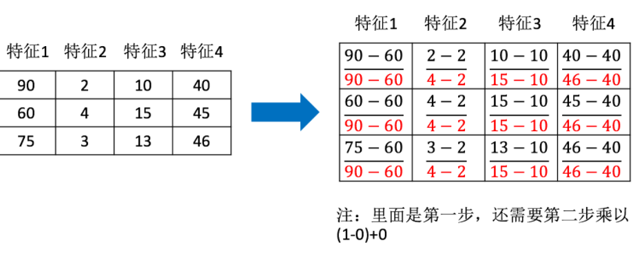
By transforming the original data, the data is mapped to (default)[0,1])between.
Formula:

understand:
Acting on each column, max Is the maximum value of a column, min Is the minimum value of a column,that X''For the final result,
mx,mi Default values for the specified interval mx Is 1,mi Is 0
Normalized API
sklearn.preprocessing.MinMaxScaler (feature_range=(0,1)... )
	MinMaxScalar.fit_transform(X)
    X:numpy array Formatted data[n_samples,n_features]
    Return value: the converted shape is the same array
Case: (appointment data)
#Part of the data. The actual data is in dating In text
milage,Liters,Consumtime,target
40920,8.326976,0.953952,3
14488,7.153469,1.673904,2
26052,1.441871,0.805124,1
75136,13.147394,0.428964,1
38344,1.669788,0.134296,1
import pandas as pd
from sklearn.preprocessing import MinMaxScaler

def minmax_demo():
    """
    Normalization demonstration
    :return: None
    """
    data = pd.read_csv("dating.txt")
    print(data)
    # 1. Instantiate a converter class
    transfer = MinMaxScaler(feature_range=(2, 3))
    # 2. Call fit_transform
    data = transfer.fit_transform(data[['milage','Liters','Consumtime']])
    print("Results of normalization of minimum and maximum values:\n", data)

    return None
Return result:
milage     Liters  Consumtime  target
0     40920   8.326976    0.953952       3
1     14488   7.153469    1.673904       2
2     26052   1.441871    0.805124       1
3     75136  13.147394    0.428964       1
..      ...        ...         ...     ...
998   48111   9.134528    0.728045       3
999   43757   7.882601    1.332446       3

[1000 rows x 4 columns]
Results of normalization of minimum and maximum values:
 [[ 2.44832535  2.39805139  2.56233353]
 [ 2.15873259  2.34195467  2.98724416]
 [ 2.28542943  2.06892523  2.47449629]
 ...,
 [ 2.29115949  2.50910294  2.51079493]
 [ 2.52711097  2.43665451  2.4290048 ]
 [ 2.47940793  2.3768091   2.78571804]]
Note: the maximum and minimum values vary. In addition, the maximum and minimum values are very vulnerable to outliers, so this method has poor robustness and is only suitable for traditional accurate small data scenarios.
2.5.3 standardization
Through the transformation of the original data, the data is transformed into the range of mean value 0 and standard deviation 1.
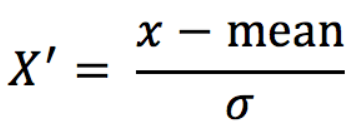
For normalization: if there are outliers that affect the maximum and minimum values, the results will obviously change
For Standardization: if there are outliers, due to a certain amount of data, a small number of outliers have little impact on the average value, so the variance change is small.
Standardized API
sklearn.preprocessing.StandardScaler( )
	·After processing, for each column, all data are clustered around the mean value 0, and the standard deviation is 1
	·StandardScaler.fit_transform(X)
	·X:numpy array Formatted data[n_samples,n_features]
	·Return value: the converted shape is the same array
Standardize the above data
import pandas as pd
from sklearn.preprocessing import StandardScaler

def stand_demo():
    """
    Standardized demonstration
    :return: None
    """
    data = pd.read_csv("dating.txt")
    print(data)
    # 1. Instantiate a converter class
    transfer = StandardScaler()
    # 2. Call fit_transform
    data = transfer.fit_transform(data[['milage','Liters','Consumtime']])
    print("Standardized results:\n", data)
    print("Average value of characteristics of each column:\n", transfer.mean_)
    print("Variance of characteristics of each column:\n", transfer.var_)

    return None
Return result:
      milage     Liters  Consumtime  target
0     40920   8.326976    0.953952       3
1     14488   7.153469    1.673904       2
2     26052   1.441871    0.805124       1
..      ...        ...         ...     ...
997   26575  10.650102    0.866627       3
998   48111   9.134528    0.728045       3
999   43757   7.882601    1.332446       3

[1000 rows x 4 columns]
Standardized results:
 [[ 0.33193158  0.41660188  0.24523407]
 [-0.87247784  0.13992897  1.69385734]
 [-0.34554872 -1.20667094 -0.05422437]
 ...,
 [-0.32171752  0.96431572  0.06952649]
 [ 0.65959911  0.60699509 -0.20931587]
 [ 0.46120328  0.31183342  1.00680598]]
Average value of characteristics of each column:
 [  3.36354210e+04   6.55996083e+00   8.32072997e-01]
Variance of characteristics of each column:
 [  4.81628039e+08   1.79902874e+01   2.46999554e-01]
**Note: * * it is relatively stable when there are enough samples, which is suitable for modern noisy big data scenarios.
2.6 feature dimensionality reduction
2.6.1 what is dimensionality reduction
Dimensionality reduction refers to the process of reducing the number of random variables (characteristics) under certain limited conditions to obtain a group of "irrelevant" main variables
It mainly reduces the number of random variables and related characteristics
Why should dimension be reduced by 6.2
It is precisely because in training, we all use features for learning. If the features have problems or the correlation between features is strong, it will have a great impact on the algorithm learning and prediction
There are two ways:
Feature selection, principal component analysis
2.6.3 feature selection
What is feature selection:
The data contains redundant or irrelevant variables (or features, attributes, indicators, etc.) in order to find out the main features from the original features.
method:
Filter(Filter type): It mainly explores the characteristics of the feature itself, the relationship between the feature and the feature and the target value
 Variance selection method: low variance feature filtering
 correlation coefficient
Embedded (Embedded): Algorithm automatically selects features (association between features and target values)
Decision tree:Information entropy, information gain
 Regularization: L1,L2
 Deep learning: convolution, etc
Filter type:
Delete some features of low variance, and then consider the angle of this method in combination with the size of variance.
Small characteristic variance: the values of most samples of a certain characteristic are relatively similar
 Large characteristic variance: the values of many samples of a certain characteristic are different
API
sklearn.feature_selection.VarianceThreshold(threshold = 0.0)
	Delete all low variance features
	Variance.fit_transform(X)
	X:numpy array Formatted data[n_samples,n_features]
	Return value: the training set difference is lower than threshold The feature will be deleted. The default value is to retain all non-zero variance features, that is, delete features with the same value in all samples.
Case: (stock data)
index,pe_ratio,pb_ratio,market_cap,return_on_asset_net_profit,du_return_on_equity,ev,earnings_per_share,revenue,total_expense,date,return
0,000001.XSHE,5.9572,1.1818,85252550922.0,0.8008,14.9403,1211444855670.0,2.01,20701401000.0,10882540000.0,2012-01-31,0.027657228229937388
1,000002.XSHE,7.0289,1.588,84113358168.0,1.6463,7.8656,300252061695.0,0.326,29308369223.2,23783476901.2,2012-01-31,0.08235182370820669
2,000008.XSHE,-262.7461,7.0003,517045520.0,-0.5678,-0.5943,770517752.56,-0.006,11679829.03,12030080.04,2012-01-31,0.09978900335112327
3,000060.XSHE,16.476,3.7146,19680455995.0,5.6036,14.617,28009159184.6,0.35,9189386877.65,7935542726.05,2012-01-31,0.12159482758620697
4,000069.XSHE,12.5878,2.5616,41727214853.0,2.8729,10.9097,81247380359.0,0.271,8951453490.28,7091397989.13,2012-01-31,-0.0026808154146886697
analysis:
1. Initialize VarianceThreshold
2. Call fit_transform
def variance_demo():
    """
    Delete low variance feature - feature selection
    :return: None
    """
    data = pd.read_csv("factor_returns.csv")
    print(data)
    # 1. Instantiate a converter class
    transfer = VarianceThreshold(threshold=1)
    # 2. Call fit_transform
    data = transfer.fit_transform(data.iloc[:, 1:10])
    print("Results of deleting low variance features:\n", data)
    print("Shape:\n", data.shape)

    return None
2.6.4 correlation coefficient
Pearson correlation coefficient(Pearson Correlation Coefficient)
	·Statistical indicators reflecting the close relationship between variables
Just know the formula:

characteristic:
The value of the correlation coefficient is between–1 And+1 Between, i.e–1≤ r ≤+1. Its nature is as follows:
When r>0 When, it indicates that the two variables are positively correlated, r<0 The two variables are negatively correlated
 When|r|=1 When, it means that the two variables are completely correlated r=0 When, it indicates that there is no correlation between the two variables
 When 0<|r|<1 It indicates that there is a certain degree of correlation between the two variables. And|r|The closer to 1, the closer the linear relationship between the two variables;|r|The closer to 0, the weaker the linear correlation between the two variables
 Generally, it can be divided into three levels:|r|<0.4 Low correlation; 0.4≤|r|<0.7 Significant correlation; 0.7≤|r|<1 It is highly linear correlation
Case: correlation calculation of financial indicators of stocks
import pandas as pd
from scipy.stats import pearsonr

def pearsonr_demo():
    """
    Correlation coefficient calculation
    :return: None
    """
    data = pd.read_csv("factor_returns.csv")

    factor = ['pe_ratio', 'pb_ratio', 'market_cap', 'return_on_asset_net_profit', 'du_return_on_equity', 'ev',
              'earnings_per_share', 'revenue', 'total_expense']

    for i in range(len(factor)):
        for j in range(i, len(factor) - 1):
            print(
                "index%s And indicators%s The correlation between is%f" % (factor[i], factor[j + 1], pearsonr(data[factor[i]], data[factor[j + 1]])[0]))

    return None
Return partial results:
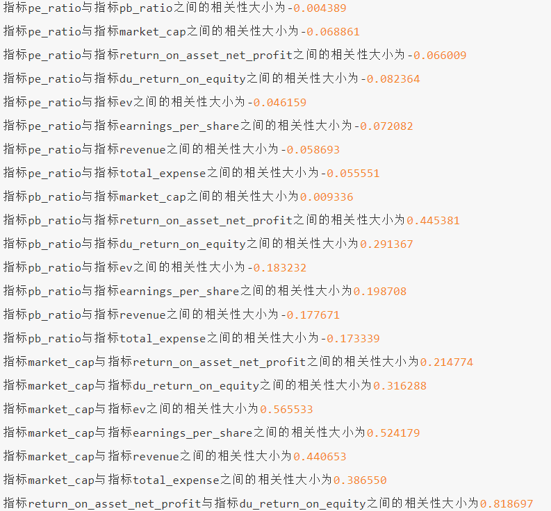
We can draw pictures and observe the results through matplotlib
2.7 principal component analysis (PCA)
2.7.1 what is principal component analysis
Definition: the process of transforming high-dimensional data into low-dimensional data. In this process, the original data may be abandoned and new variables may be created

Function: it is data dimension compression to reduce the dimension (complexity) of the original data as much as possible and lose a small amount of information.

Application: regression analysis or cluster analysis
API
sklearn.decomposition.PCA(n_components=None)
	Decompose data into lower dimensional space
	n_components:
		Decimal: indicates the percentage of information retained
		Integer: reduce to how many characteristics
	PCA.fit_transform(X) X:numpy array Formatted data[n_samples,n_features]
		Return value: the value of the specified dimension after conversion array
Case: Explore Users' preferences for item categories, subdivide and reduce dimensions
The data are as follows:
order_products__prior.csv: Order and product information
 Field: order_id, product_id, add_to_cart_order, reordered

products.csv: Commodity information
 Field: product_id, product_name, aisle_id, department_id

orders.csv: User's order information
 Field: order_id,user_id,eval_set,order_number,....

aisles.csv: Specific item category of commodity
 Field: aisle_id, aisle
analysis:
1.Consolidate tables so that user_id And aisle In a table
2.Perform crosstab transformation
3.Dimensionality reduction
import pandas as pd
from sklearn.decomposition import PCA

# 1. Get dataset
# ·Product information - products csv:
# Fields: product_id, product_name, aisle_id, department_id
# ·Order and product information - order_products__prior.csv:
# Fields: order_id, product_id, add_to_cart_order, reordered
# ·User's order information - orders csv:
# Fields: order_id, user_id,eval_set, order_number,order_dow, order_hour_of_day, days_since_prior_order
# ·Specific item category of goods - aisles csv:
# Fields: aisle_id, aisle
products = pd.read_csv("./instacart/products.csv")
order_products = pd.read_csv("./instacart/order_products__prior.csv")
orders = pd.read_csv("./instacart/orders.csv")
aisles = pd.read_csv("./instacart/aisles.csv")

# 2. Merge tables, user_id and aisle are put on one table
# 1) Merge orders and order_products on=order_id tab1:order_id, product_id, user_id
tab1 = pd.merge(orders, order_products, on=["order_id", "order_id"])
# 2) Merge tab1 and products on=product_id tab2:aisle_id
tab2 = pd.merge(tab1, products, on=["product_id", "product_id"])
# 3) Merge tab2 and aisles on=aisle_id tab3:user_id, aisle
tab3 = pd.merge(tab2, aisles, on=["aisle_id", "aisle_id"])

# 3. Cross table processing_ ID and aisle are grouped
table = pd.crosstab(tab3["user_id"], tab3["aisle"])

# 4. Principal component analysis is used to reduce dimension
# 1) Instantiate a converter class PCA
transfer = PCA(n_components=0.95) #Retain 95% of information
# 2)fit_transform
data = transfer.fit_transform(table)

print(data.shape)
Return result:
(206209, 44)
III. summary chart
